Hong Hao: Outlook 2019: Turning a Corner
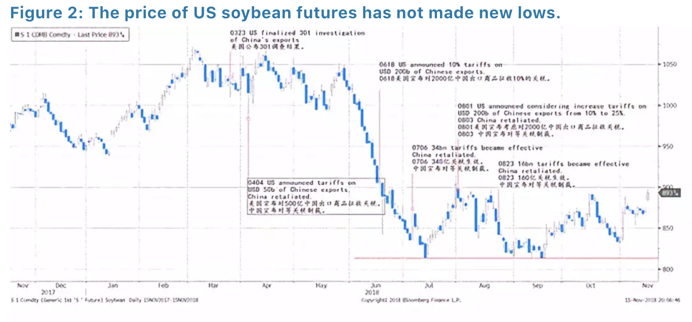
2018-11-27 IMI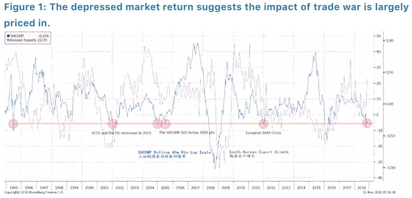 Another way to investigate the impact of the trade war is to look at the price of soybean futures – a commodity directly affected by the trade war due to its importance in US exports to China, as well as the Midwest’s sway in the US election. We note that the price of US soybean futures has stopped making new lows in recent months, even as the prospects of the trade war worsen (Figure 2). This observation shows that the market has largely priced in the near-term impact of the trade war. Both the Shanghai Composite and the US soybean futures are hinting at the likelihood of a truce in terms of market price for now. It is constructive that both sides are starting to talk again.
 TWO: Three Balance Sheets in China’s Economy
Our economic cycle model shows that China’sshort economic cycle will likely trough in the coming months, given the right mix of fiscal stimulus and monetary easing. Our cycle model also shows that theUS short economic cycle is peaking, and will likely continue to stir overseas markets in the near term (please refer to our report “The Colliding Cycles of China and the US” on 20180903).
When the economic cycle is approaching its upturning point, it means that the pendulum of negativity in the economy has swung too far. At this point, one can observe that credit expansion has slowed to a level below the nominal economic growth, despite falling interest rate; economic activities, notably building construction in China, are grinding to a halt; consumption is weak and inventory level is low. The stock market, one of the most watched barometers of economic activities, is depressed. China is now at this juncture.
However, for an economic cycle to turn up, help from government policy is often required. And the greater the challenges, the higher the intensity of policy support should be – as now. The condition for the policies to be effective, is that the government still has leeway to stimulate, and the private sector’s balance sheet is not leveraged to a point that is beyond repair. In short, there should still be room to transfer the burden of leverage between the public and private balance sheets.
In the following sections, we investigate the state of leverage in different parts of China’s economy.
Household: China’s Property Bubble – A Different Perspective
Is China’s property a bubble? This debate has not been settled - yet. Critics, including myself, have been applying extremely low rental yields versus mortgage rate, high ratio of property price to income and vacancy rate to justify their view of a property bubble. Yet, China’s property price continues to surge, despite these elaborate and thoughtful arguments. Although property is an asset of long duration and thus it is difficult to time the exit, such price performance suggests that the prevailing arguments may be too early to be right.
As the Chinese economy decelerates, and pressure on property price becomes increasingly palpable, the focus of the debate has turned to whether high property price has obliged Chinese households to take on leverage to an unsustainably high level, and has affected consumption. And eventually, such unsustainable leverage may lead to a bust of the property bubble.
Besides the conventional metrics of measuring housing affordability and the health of household balance sheet, we believe that it is more pertinent to check the debt service ratio of Chinese households over time and on a regional basis. The logic is that if the Chinese households can service their mortgage, then as long as return on property purchase exceeds mortgage rate, it is indeed rational to take on leverage. And as the property market varies between regions, it pays to look at regional differences.
TWO: Three Balance Sheets in China’s Economy
Our economic cycle model shows that China’sshort economic cycle will likely trough in the coming months, given the right mix of fiscal stimulus and monetary easing. Our cycle model also shows that theUS short economic cycle is peaking, and will likely continue to stir overseas markets in the near term (please refer to our report “The Colliding Cycles of China and the US” on 20180903).
When the economic cycle is approaching its upturning point, it means that the pendulum of negativity in the economy has swung too far. At this point, one can observe that credit expansion has slowed to a level below the nominal economic growth, despite falling interest rate; economic activities, notably building construction in China, are grinding to a halt; consumption is weak and inventory level is low. The stock market, one of the most watched barometers of economic activities, is depressed. China is now at this juncture.
However, for an economic cycle to turn up, help from government policy is often required. And the greater the challenges, the higher the intensity of policy support should be – as now. The condition for the policies to be effective, is that the government still has leeway to stimulate, and the private sector’s balance sheet is not leveraged to a point that is beyond repair. In short, there should still be room to transfer the burden of leverage between the public and private balance sheets.
In the following sections, we investigate the state of leverage in different parts of China’s economy.
Household: China’s Property Bubble – A Different Perspective
Is China’s property a bubble? This debate has not been settled - yet. Critics, including myself, have been applying extremely low rental yields versus mortgage rate, high ratio of property price to income and vacancy rate to justify their view of a property bubble. Yet, China’s property price continues to surge, despite these elaborate and thoughtful arguments. Although property is an asset of long duration and thus it is difficult to time the exit, such price performance suggests that the prevailing arguments may be too early to be right.
As the Chinese economy decelerates, and pressure on property price becomes increasingly palpable, the focus of the debate has turned to whether high property price has obliged Chinese households to take on leverage to an unsustainably high level, and has affected consumption. And eventually, such unsustainable leverage may lead to a bust of the property bubble.
Besides the conventional metrics of measuring housing affordability and the health of household balance sheet, we believe that it is more pertinent to check the debt service ratio of Chinese households over time and on a regional basis. The logic is that if the Chinese households can service their mortgage, then as long as return on property purchase exceeds mortgage rate, it is indeed rational to take on leverage. And as the property market varies between regions, it pays to look at regional differences.
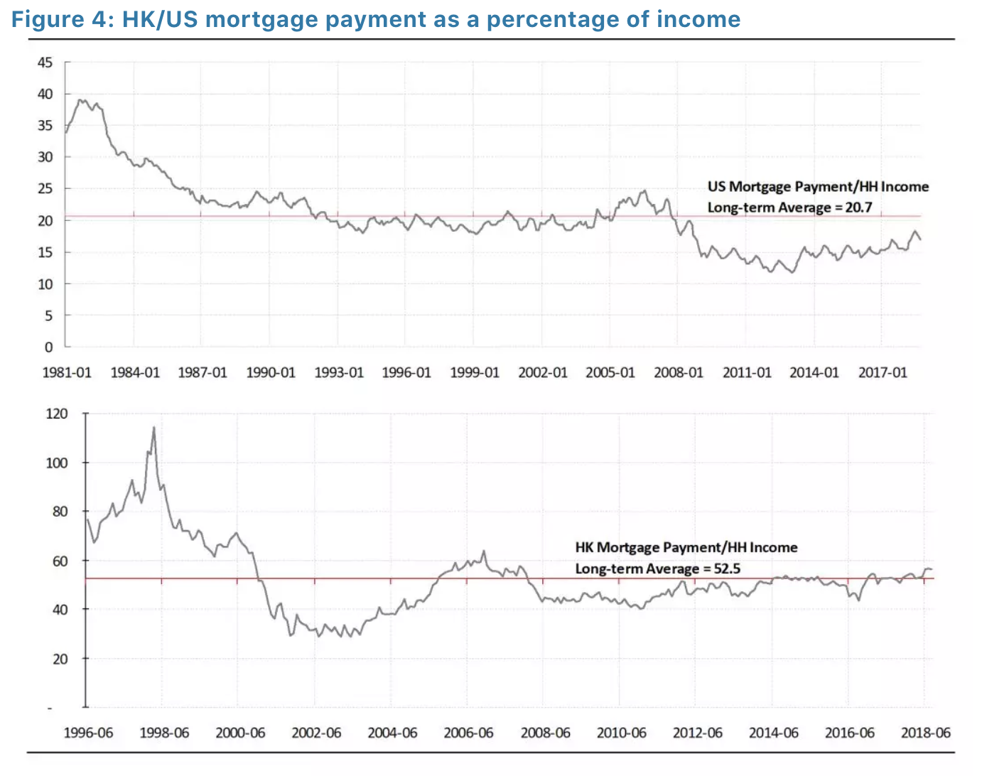
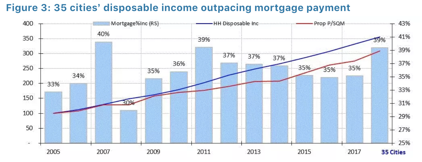 We find that, on a national level, household disposable income had outpaced property price appreciation. Mortgage payment as a percentage of household income is 39%. This ratio has risen to close to the highest level last seen in 2007 and 2011 – both followed by difficult years for China’s economy (Figure 3). Compared with 21% in the US where interest rate is starting to rise from historic lows, this ratio may suggest that the Chinese households are heavily in debt. But it compares favorably with that of Hong Kong at 56%, and Hong Kong’s ratio was higher than 100% during the bubble years of 1997. As such, there appears to be a cultural difference between the east and the west (Figure 4).
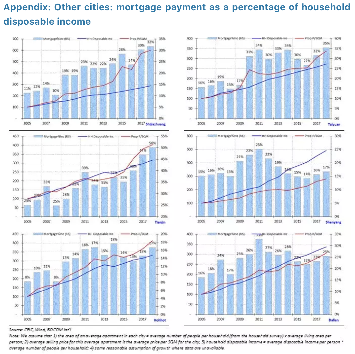
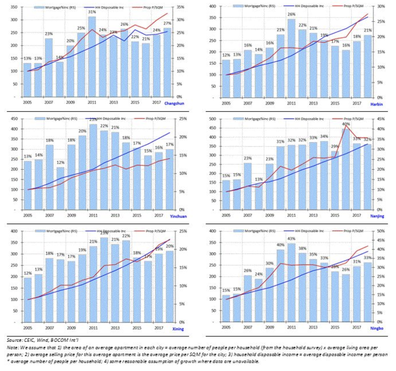
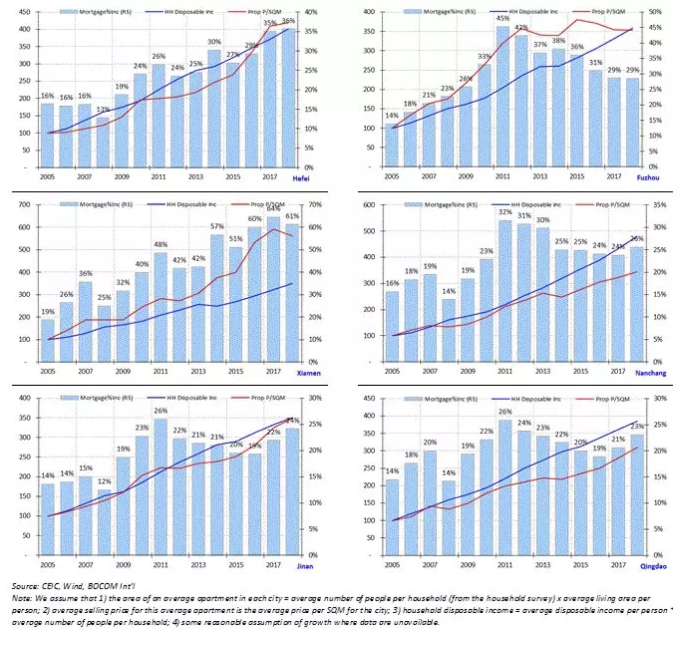
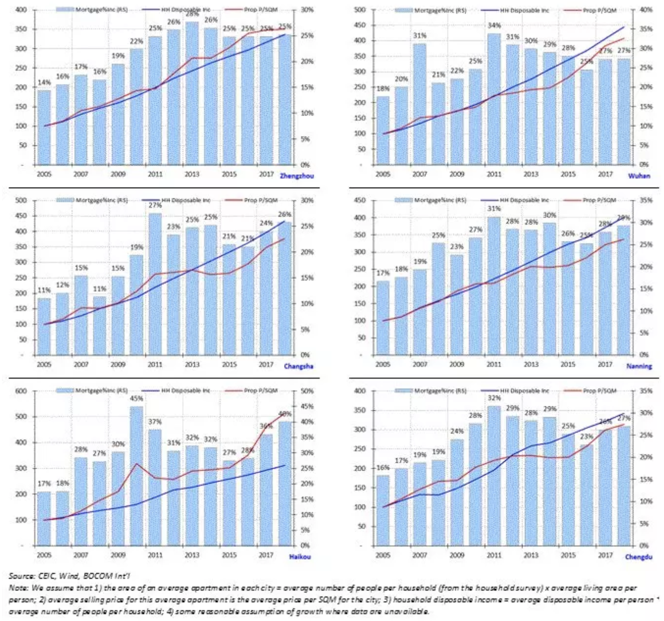
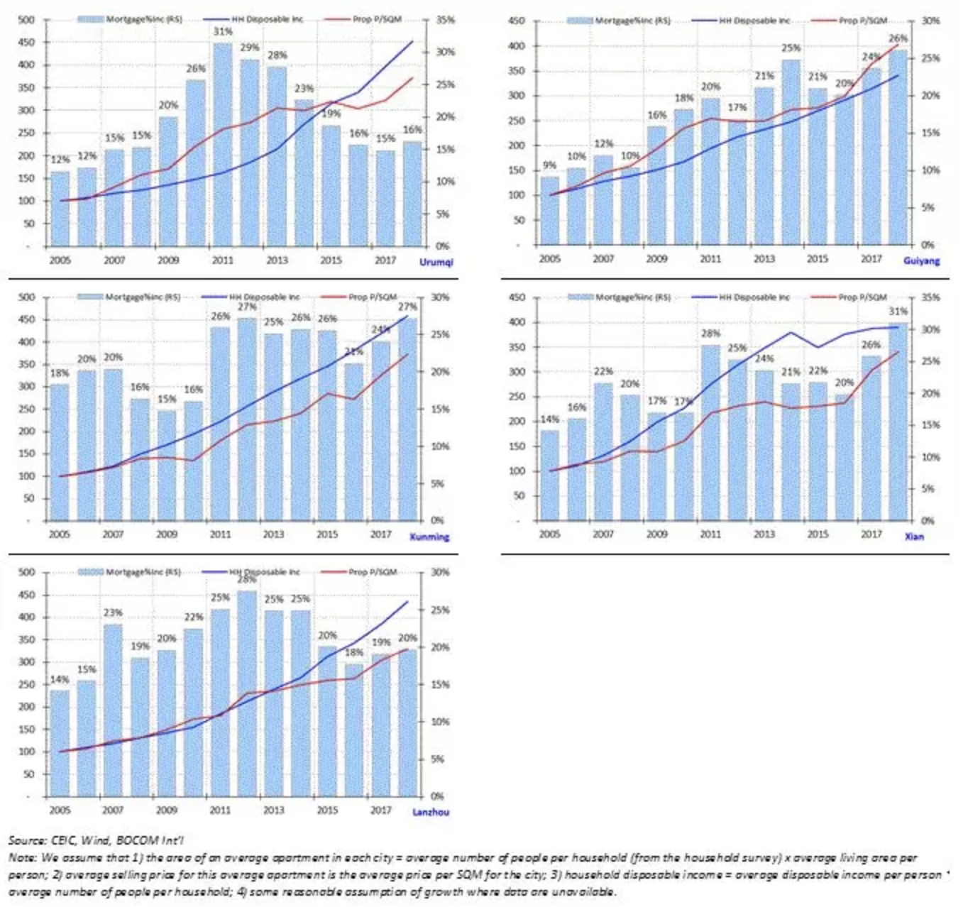
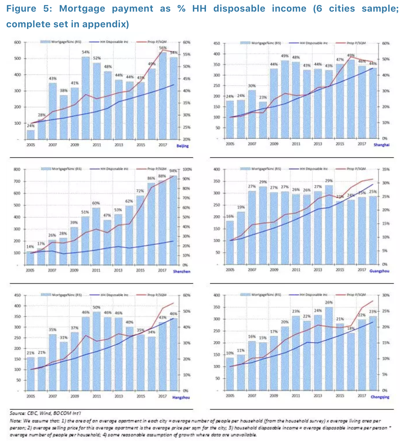
 We apply the same methodology to calculate the mortgage service ratios of 35 major Chinese cities, with some reasonable assumptions (Figure 5 shows a sample of cities; for presentation purpose, the rest please refer to appendix at the back of this report). We find that only 16 out of 35 major cities have seen household disposable income rising faster than property price since 2005. And all Tier-1 cities except Guangzhou have experienced faster property price growth than that of household income, respectively. That is, on a regional basis, the Chinese property bubble is concerning, if such trends persist.
 In sum, we conclude that the Chinese households’ ability to service their mortgages has deteriorated to the level similar to 2007 and 2011, two of the years followed by difficult property market conditions in 2008 and 2012. These years also coincide with the last year of the short economic cycle in the US, which we will discuss later in the report. As a whole, the Chinese households’ balance sheet is highly leveraged, but is not yet on the brink of collapse – judging from the mortgage service ability.
Local Government Debt Woes
Can local governments go on with their increasing debt load? It has been a pesky concern for investors. Local government debt problems first surfaced in 2010, after the four-trillion-yuan stimulus in 2009. I still remember leading an investor group to conduct due diligence on local governments up and down the Yangtze back then. Recently, with headlines such as some counties failing to pay public servants’ stipends, the concerns on local government debts grow louder.
The challenge of analyzing local government debt lies in its transparency. Reliable data are hard to come by. And the LGFV and hidden liabilities via implicit debt guarantee for companies owned by or associated with local governments present further complications.
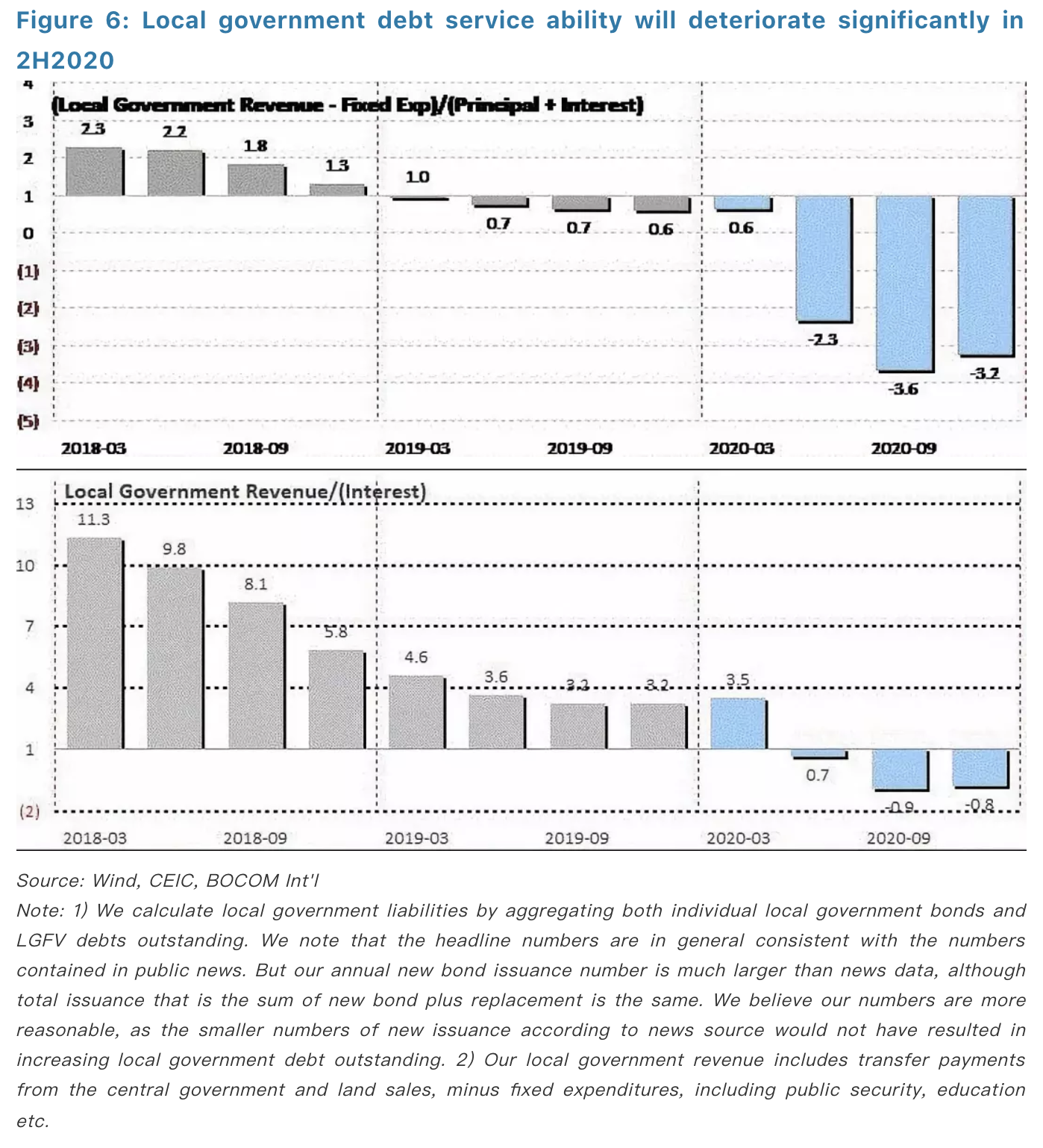
Our methodology is to use the bond data, of both local government bonds and the LGFV debt, to aggregate the apparent liabilities of local governments from bottom up. Such data include principal maturity and periodical interest payment information. We then compare these aggregated numbers with the numbers in sporadic news and national audits to verify their legitimacy. Obviously, our analysis does not include the implicit liabilities aforementioned. As the fiscal deficit on the central government level is still considered low at 2.7%, versus the international standard of 3%, we can save time by focusing on the local governments. We consider our analysis the best-case scenario analysis, as it includes only apparent liabilities and ignores potential new issuance from now (Figure 6).
We find that local governments’ ability to service debt, after deducting its responsibilities of fixed expenditures such as providing public security and education, will be tipped to negative in 2019. But it will deteriorate significantly in 2H2020, as the large amount of bonds issued in the past three years come due.
We can assume that these bonds will be rolled over when they mature in 2020. But such a maneuver will increase local governments’ leverage even further. If we assume all these bonds can be paid off by transfer payments from the central government, it will increase central fiscal deficit to close to 4%.
If we assume all bonds maturing will be rolled over by issuing new debt, then the picture of local government debt service ability will improve greatly. Even so, local governments will still find it difficult to finance its liabilities in 2H2020. Either way, it is a monumental challenge. Fortunately, it is not yet an immediate threat.
In sum, we conclude that the Chinese households’ ability to service their mortgages has deteriorated to the level similar to 2007 and 2011, two of the years followed by difficult property market conditions in 2008 and 2012. These years also coincide with the last year of the short economic cycle in the US, which we will discuss later in the report. As a whole, the Chinese households’ balance sheet is highly leveraged, but is not yet on the brink of collapse – judging from the mortgage service ability.
Local Government Debt Woes
Can local governments go on with their increasing debt load? It has been a pesky concern for investors. Local government debt problems first surfaced in 2010, after the four-trillion-yuan stimulus in 2009. I still remember leading an investor group to conduct due diligence on local governments up and down the Yangtze back then. Recently, with headlines such as some counties failing to pay public servants’ stipends, the concerns on local government debts grow louder.
The challenge of analyzing local government debt lies in its transparency. Reliable data are hard to come by. And the LGFV and hidden liabilities via implicit debt guarantee for companies owned by or associated with local governments present further complications.
Our methodology is to use the bond data, of both local government bonds and the LGFV debt, to aggregate the apparent liabilities of local governments from bottom up. Such data include principal maturity and periodical interest payment information. We then compare these aggregated numbers with the numbers in sporadic news and national audits to verify their legitimacy. Obviously, our analysis does not include the implicit liabilities aforementioned. As the fiscal deficit on the central government level is still considered low at 2.7%, versus the international standard of 3%, we can save time by focusing on the local governments. We consider our analysis the best-case scenario analysis, as it includes only apparent liabilities and ignores potential new issuance from now (Figure 6).
We find that local governments’ ability to service debt, after deducting its responsibilities of fixed expenditures such as providing public security and education, will be tipped to negative in 2019. But it will deteriorate significantly in 2H2020, as the large amount of bonds issued in the past three years come due.
We can assume that these bonds will be rolled over when they mature in 2020. But such a maneuver will increase local governments’ leverage even further. If we assume all these bonds can be paid off by transfer payments from the central government, it will increase central fiscal deficit to close to 4%.
If we assume all bonds maturing will be rolled over by issuing new debt, then the picture of local government debt service ability will improve greatly. Even so, local governments will still find it difficult to finance its liabilities in 2H2020. Either way, it is a monumental challenge. Fortunately, it is not yet an immediate threat.
 Corporate Leverage Problems
Recently, concerns have arisen over potential “fall-back” of private companies in China to state ownership, if the market turmoil continues. Many critics point to the diverging financial performances between state-owned and private enterprises in the manufacturing sector as the evidence of the malaise that private firms are suffering.
While these concerns are not without their merits, the manufacturing sector is only one part of the Chinese economy that is restructuring towards a consumption-led economy. Further, SOEs have natural advantages in this capital-intensive sector consisting of many upstream commodity producers. These sectors have strengthened during the supply-side reform. As such, using only the developments in the manufacturing sectors is tantamount to taking a few trees for the forest.
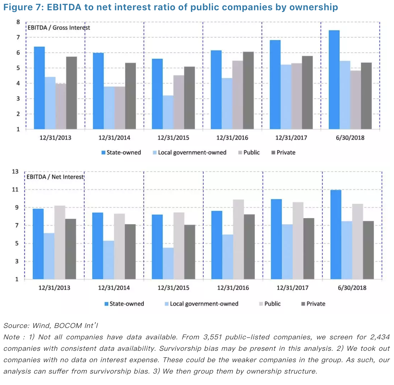
Once again, we analyze public companies’ debt service ability by measuring their EBITDA-Net interest coverage ratio. We aggregate public companies’ financial data from bottom up, and group them by ownership structure. Indeed, we find that the ability of state-owned and local government-owned companies to service debt has improved in the past five years, while that of private companies has deteriorated somewhat. That said, the net interest coverage ratio is still reasonable for private companies (Figure 7).
Recently, there have been concerns about the selling pressure induced by share pledge loans. Our quantitative analysis shows that the amount of shares pledged and the percentage of total market capitalization pledged have been rising since early 2015; even the stock market bubble burst only managed to put a fleeting dent in the share-pledge practice. The percentage of the market cap pledged had risen until March 2018, and then began to fall sharply. It appears that, as the market plunge accelerated, margin calls on shares pledged increased – it was like stepping on the gas pedal.
That said, given that the entire emerging market has been under pressure since late January, and that the percentage of market cap pledged has been rising in tandem as the market recovered from the 2015 crash, it is unlikely that these share-pledged loans are the reason for the bear market, although they must have aggravated it. Meanwhile, the surging volatility in the US market has not helped – the consequence of the colliding economic down-cycle in China and the peaking cycle in the US. We will discuss these cycles in the later section of this report.
Corporate Leverage Problems
Recently, concerns have arisen over potential “fall-back” of private companies in China to state ownership, if the market turmoil continues. Many critics point to the diverging financial performances between state-owned and private enterprises in the manufacturing sector as the evidence of the malaise that private firms are suffering.
While these concerns are not without their merits, the manufacturing sector is only one part of the Chinese economy that is restructuring towards a consumption-led economy. Further, SOEs have natural advantages in this capital-intensive sector consisting of many upstream commodity producers. These sectors have strengthened during the supply-side reform. As such, using only the developments in the manufacturing sectors is tantamount to taking a few trees for the forest.
Once again, we analyze public companies’ debt service ability by measuring their EBITDA-Net interest coverage ratio. We aggregate public companies’ financial data from bottom up, and group them by ownership structure. Indeed, we find that the ability of state-owned and local government-owned companies to service debt has improved in the past five years, while that of private companies has deteriorated somewhat. That said, the net interest coverage ratio is still reasonable for private companies (Figure 7).
Recently, there have been concerns about the selling pressure induced by share pledge loans. Our quantitative analysis shows that the amount of shares pledged and the percentage of total market capitalization pledged have been rising since early 2015; even the stock market bubble burst only managed to put a fleeting dent in the share-pledge practice. The percentage of the market cap pledged had risen until March 2018, and then began to fall sharply. It appears that, as the market plunge accelerated, margin calls on shares pledged increased – it was like stepping on the gas pedal.
That said, given that the entire emerging market has been under pressure since late January, and that the percentage of market cap pledged has been rising in tandem as the market recovered from the 2015 crash, it is unlikely that these share-pledged loans are the reason for the bear market, although they must have aggravated it. Meanwhile, the surging volatility in the US market has not helped – the consequence of the colliding economic down-cycle in China and the peaking cycle in the US. We will discuss these cycles in the later section of this report.
 THREE: The Short Cycles of the US and China
“The only thing we learn from history is that we learn nothing from history.” – Hegel
The most pressing question
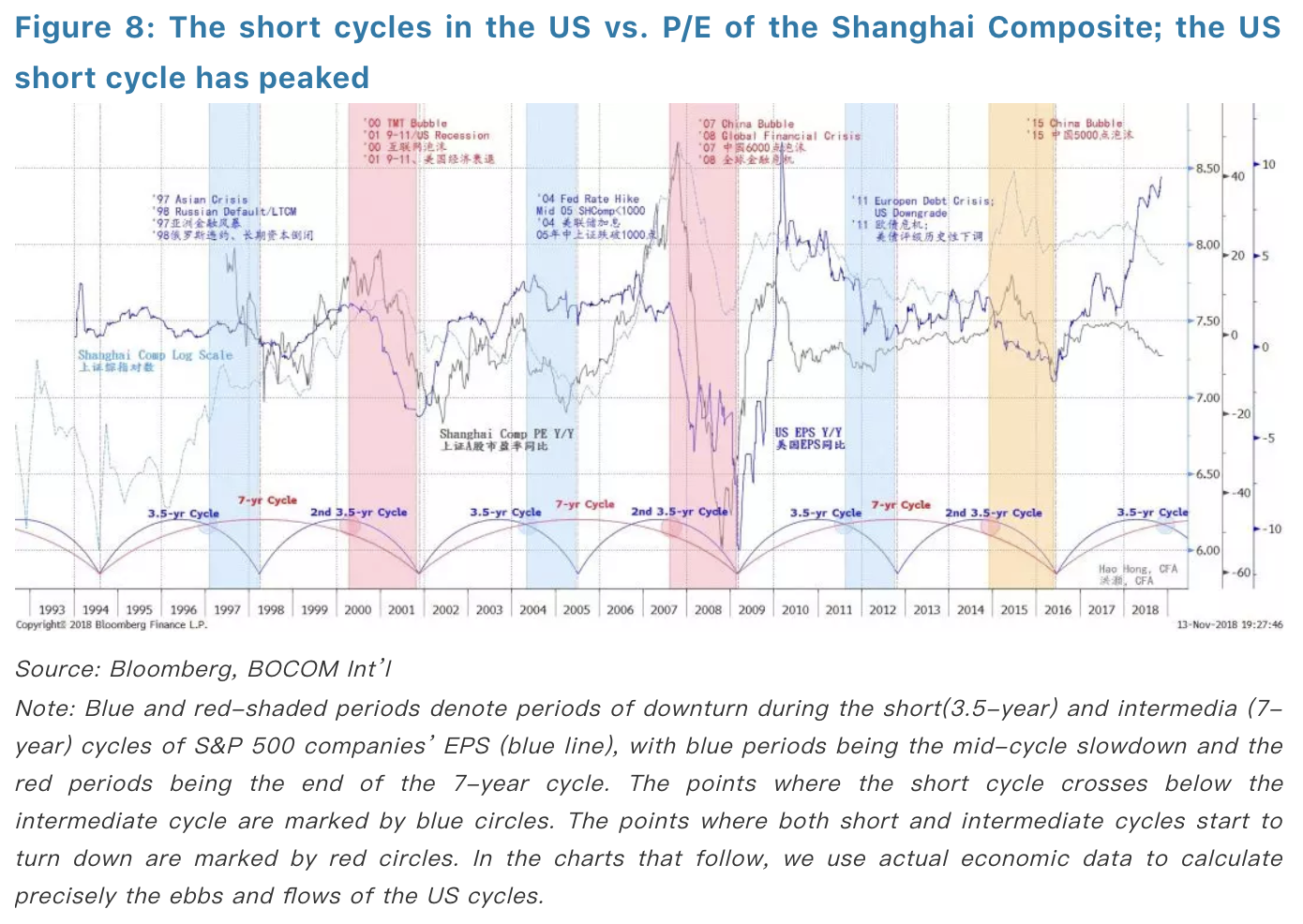
There exist a 3.5-year cycle in the US economy (Figure 8), and a 3-year cycle in China. We demonstrate in this paper as follows, with charts drawn from quantitative analysis, the cyclical character of the economies of the US and China.
After we published our first paper on economic cycles with quantitative metrics titled “A Definitive Guide to China’s Economic Cycle” (20170323), we were invited to give a public lecture on economic cycles at one of the most prestigious Chinese universities. A renowned economist, one of the finest of his kind, quipped: “Can you trade on it? How could you be sure that it will be the same next time?”
Forecast is hard, especially when it is about the future. While all models are wrong, some are useful. The significance of any cyclical model is to evaluate and forecast the underlying trend less perceptible to many, as well as the approximate timing of turning points. Such forecasts, albeit with no guarantee, improve the odds of profiting. Incidentally, we based our bearish 2018 outlook report titled “View from the Peak” (20171207) on the declining phase in China’s 3-year cycle - amid the then generally rosy consensus. Since its late January peak, the Shanghai Composite has fallen ~30%. Now the pressing question is: where is the bottom?
THREE: The Short Cycles of the US and China
“The only thing we learn from history is that we learn nothing from history.” – Hegel
The most pressing question
There exist a 3.5-year cycle in the US economy (Figure 8), and a 3-year cycle in China. We demonstrate in this paper as follows, with charts drawn from quantitative analysis, the cyclical character of the economies of the US and China.
After we published our first paper on economic cycles with quantitative metrics titled “A Definitive Guide to China’s Economic Cycle” (20170323), we were invited to give a public lecture on economic cycles at one of the most prestigious Chinese universities. A renowned economist, one of the finest of his kind, quipped: “Can you trade on it? How could you be sure that it will be the same next time?”
Forecast is hard, especially when it is about the future. While all models are wrong, some are useful. The significance of any cyclical model is to evaluate and forecast the underlying trend less perceptible to many, as well as the approximate timing of turning points. Such forecasts, albeit with no guarantee, improve the odds of profiting. Incidentally, we based our bearish 2018 outlook report titled “View from the Peak” (20171207) on the declining phase in China’s 3-year cycle - amid the then generally rosy consensus. Since its late January peak, the Shanghai Composite has fallen ~30%. Now the pressing question is: where is the bottom?
 The short cycle in the US
“When in economics we speak of cycles, we generally mean seven to eleven-year business cycles … which we shall agree to call ‘intermediate’, the existence of still shorter waves of about three and one-half years length has recently been shown to be probable... The length of the latter (intermediate waves) fluctuates at least between 7 and 11 years.” – The Long Waves in Economic Life, Nikolai D. Kondratieff
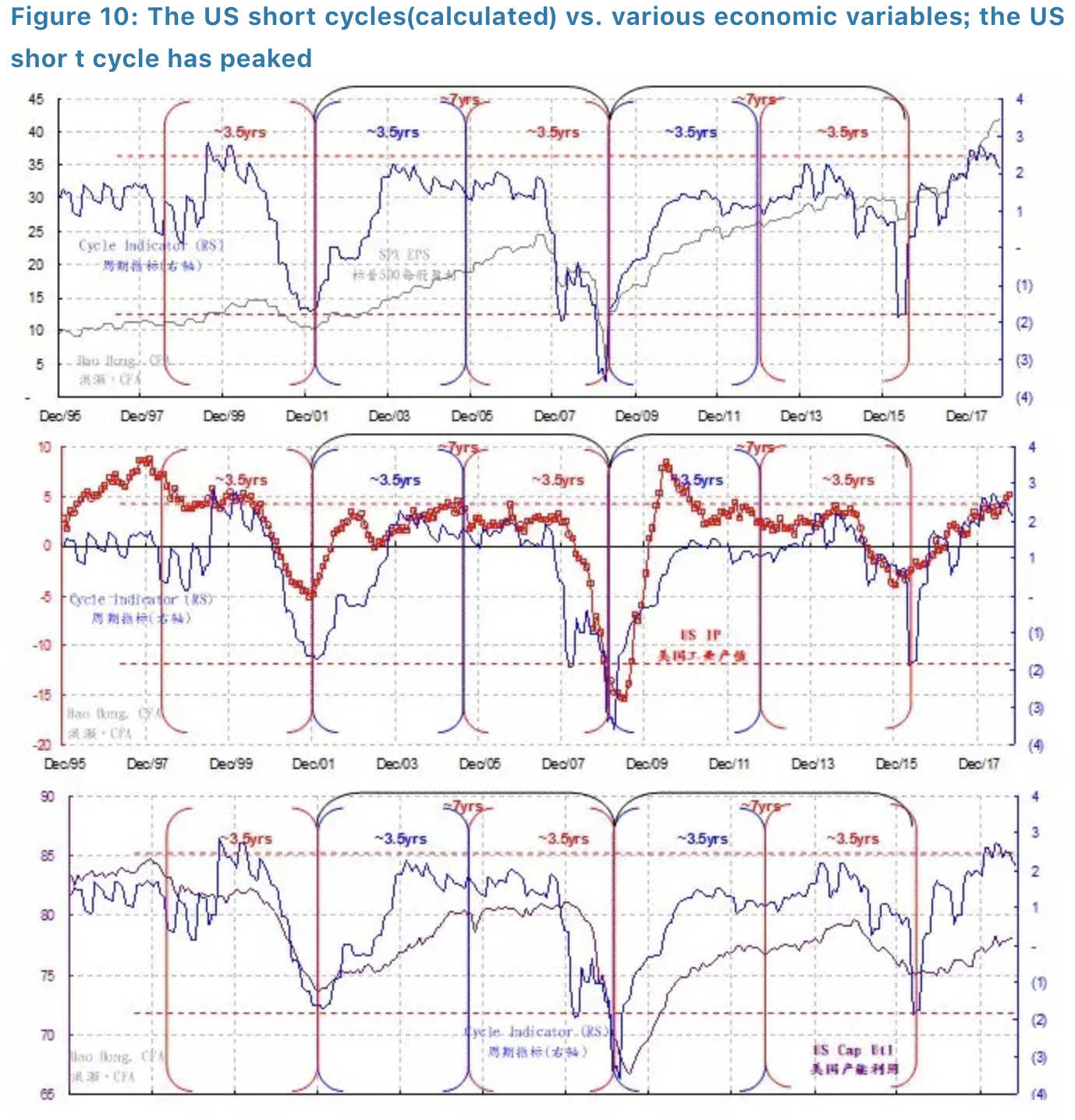
In Figure 8, we use the adjusted EPS of the S&P500 index as a proxy for the short-term fluctuations in the US economy. Our chart analysis shows that there clearly exists a 3.5-year cycle in the US economy. And two 3.5-year short cycles constitute a complete, trough-to-trough,7-year intermediate cycle. We observe the following in Figure 8:
(1)There have been six 3.5-year short cycles and three 7-year intermediate cycles since1994 (shown by blue and red arcs along the time axis at the chart bottom). Two of the most recent complete cycles run from Dec 2001 to Dec 2008, and from Dec2008 to Dec 2015, with mid-2005 and mid-2012 as the cyclical interludes, respectively.
(2)In the first 3.5-year short cycle within the 7-year intermediate cycle, when the short cycle finishes its uptrend and then crosses below the intermediate cycle(marked by blue circles), regional crises tend to be concurrent (shown and annotated in blue-shaded periods). For instance, the ’97 Asian Crisis and ’98Russian Defaults, and the European Sovereign Debt Crisis and the historic USsovereign rating downgrade in 2011. The current crises in Turkey and Argentina appear to be mid-cycle crises of such nature.
(3)In the second half of the 7-year intermediate cycle, when both the 3.5-year short cycle and the 7-year intermediate cycle start to decline (marked by red circles), crises of a more significant scale tend to happen. For instance, the burst of the TMT Bubble in 2000, the September-11 and the US recession in 2001, as well as the 2008 Global Financial Crisis (shown and annotated in red-shaded periods). Although much less discussed, the decline in the US stock market in2001 and 2008 are of similar magnitude – both had halved. These two episodes give us reasonable anchor in time to calculate the duration of the cycles. The positive influence the rising trends have on asset prices tends to last longer than the negative impact of the falling trends.
(4)History suggests that the snag that global markets are experiencing can be the last leg of an 11-year intermediate cycle consisting three 3.5-year short cycles starting from early 2009 and ending in early 2019. But it could also be the first 3.5-year short cycle within a renewed intermediate cycle of 7 years, consisting of two 3.5-year cycles and starting from early 2016. If so, the emerging turbulence ahead will bear much less significance than the end of an 11-year intermediate cycle would suggest.
(5)China’s own 3-year economic cycle is entering its last phase of decline in the coming months. This declining phase in the Chinese cycle happens to coincide with the late cycle in the US 3.5-year short cycle between 4Q18 and 1Q19, as suggested by our model (we will update our model on the Chinese economic cycle in the later part of this report). Expect significant turbulence. This coincidence can well be the reason why the Chinese stock market has been finding it hard to bottom out, albeit having cheapened substantially.
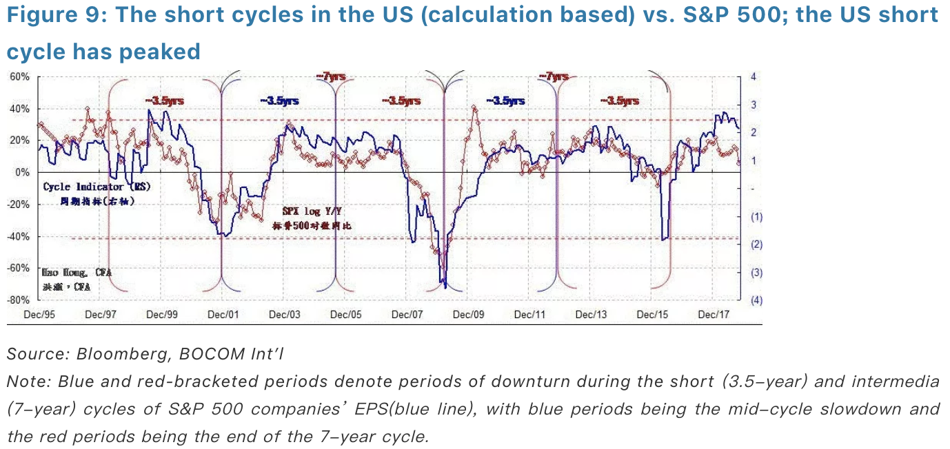
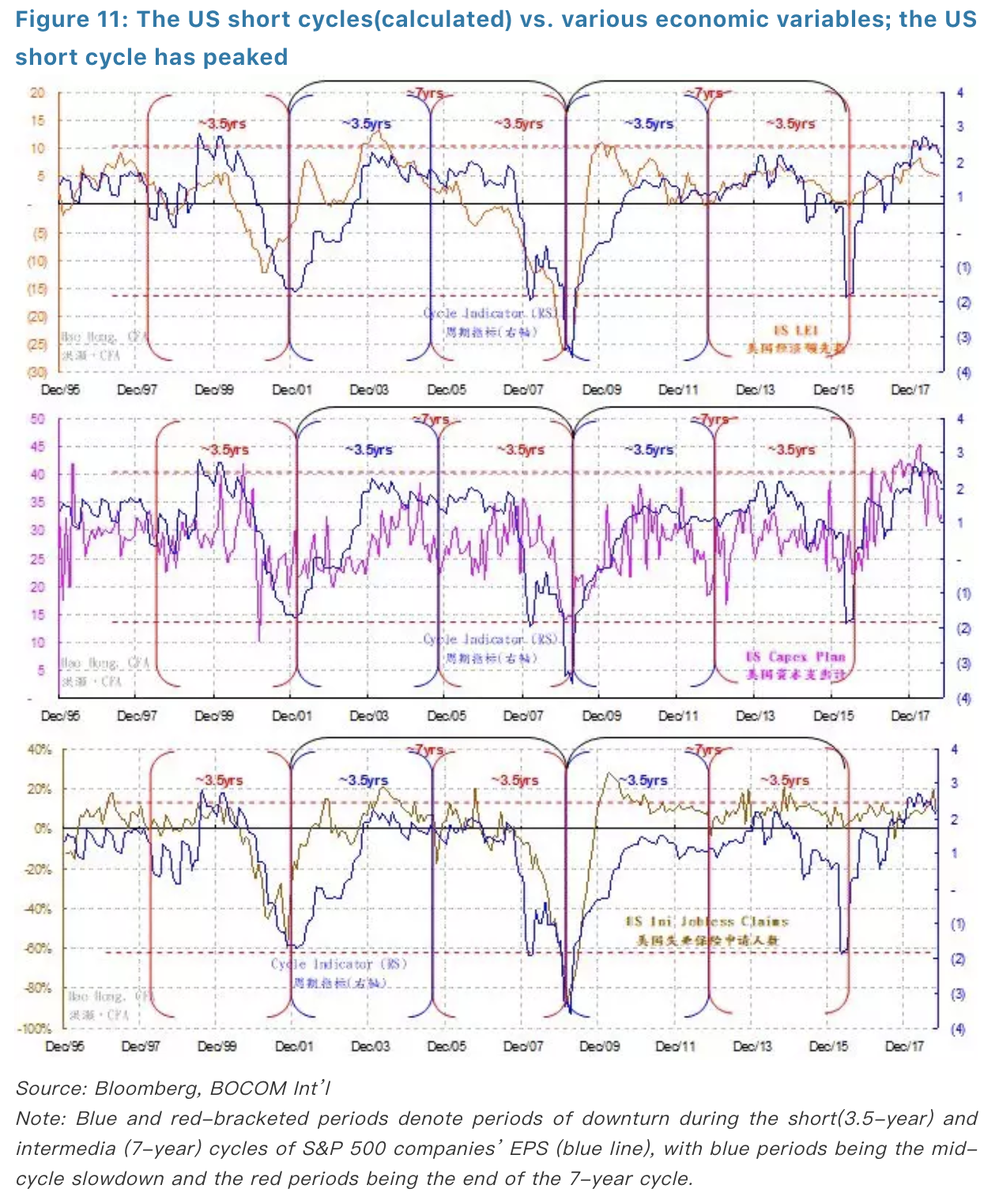
We charted Figure 8 using the Bloomberg charting tools. While intuitive and visually appealing, we need to verify its rigor with quantitative modelling. From Figure 9 to 11, we use monthly-adjusted EPSto model the short and intermediate cycles in the US economy. We can demonstrate clearly the 3.5-year short cycle, and the 7-year intermediate cycle consisting of two 3.5-year short cycles in the US economy for over two decades in the past.
We then overlay other US macroeconomic variables, such as the S&P 500 index, IP, capacity utilization, Leading Economic Indicator, capex plan and employment, with our US Cycle Indicator. Readers can see the very tight correlation between these variables and the Cycle Indicator.
Note that these correlations amongst market price, output, volume or surveys testify the validity of our cyclical model: the cycles identified here cannot be simply dismissed as happenstances. All of these important time series exhibit well-defined time duration of similar length. And their important turning points largely correspond, despite the complicated statistical and mathematical treatments of these data.
Deviation from general rules that prevails in the sequence of the cycles is very rare. Even when there is deviation from the underlying trend, such deviation tends to accelerate or retard its own momentum, rather than that of the underlying trends. The absence of such deviation is also are markable proof of the cycle’s existence.
Indeed, the 3.5-year short cycle in the US economy is consistent with the 3-year cycle in China’s economy that we identified in our previous report titled “A definitive guide to China’s Economic Cycle” (20170323). The intermediate cycles of six to seven years consisting of two short cycles in these two economies are also consistent. These entwining short and intermediate cycles between the US andChina must have profound implications on economic and market performances, as well as policy choices.
The short cycle in the US
“When in economics we speak of cycles, we generally mean seven to eleven-year business cycles … which we shall agree to call ‘intermediate’, the existence of still shorter waves of about three and one-half years length has recently been shown to be probable... The length of the latter (intermediate waves) fluctuates at least between 7 and 11 years.” – The Long Waves in Economic Life, Nikolai D. Kondratieff
In Figure 8, we use the adjusted EPS of the S&P500 index as a proxy for the short-term fluctuations in the US economy. Our chart analysis shows that there clearly exists a 3.5-year cycle in the US economy. And two 3.5-year short cycles constitute a complete, trough-to-trough,7-year intermediate cycle. We observe the following in Figure 8:
(1)There have been six 3.5-year short cycles and three 7-year intermediate cycles since1994 (shown by blue and red arcs along the time axis at the chart bottom). Two of the most recent complete cycles run from Dec 2001 to Dec 2008, and from Dec2008 to Dec 2015, with mid-2005 and mid-2012 as the cyclical interludes, respectively.
(2)In the first 3.5-year short cycle within the 7-year intermediate cycle, when the short cycle finishes its uptrend and then crosses below the intermediate cycle(marked by blue circles), regional crises tend to be concurrent (shown and annotated in blue-shaded periods). For instance, the ’97 Asian Crisis and ’98Russian Defaults, and the European Sovereign Debt Crisis and the historic USsovereign rating downgrade in 2011. The current crises in Turkey and Argentina appear to be mid-cycle crises of such nature.
(3)In the second half of the 7-year intermediate cycle, when both the 3.5-year short cycle and the 7-year intermediate cycle start to decline (marked by red circles), crises of a more significant scale tend to happen. For instance, the burst of the TMT Bubble in 2000, the September-11 and the US recession in 2001, as well as the 2008 Global Financial Crisis (shown and annotated in red-shaded periods). Although much less discussed, the decline in the US stock market in2001 and 2008 are of similar magnitude – both had halved. These two episodes give us reasonable anchor in time to calculate the duration of the cycles. The positive influence the rising trends have on asset prices tends to last longer than the negative impact of the falling trends.
(4)History suggests that the snag that global markets are experiencing can be the last leg of an 11-year intermediate cycle consisting three 3.5-year short cycles starting from early 2009 and ending in early 2019. But it could also be the first 3.5-year short cycle within a renewed intermediate cycle of 7 years, consisting of two 3.5-year cycles and starting from early 2016. If so, the emerging turbulence ahead will bear much less significance than the end of an 11-year intermediate cycle would suggest.
(5)China’s own 3-year economic cycle is entering its last phase of decline in the coming months. This declining phase in the Chinese cycle happens to coincide with the late cycle in the US 3.5-year short cycle between 4Q18 and 1Q19, as suggested by our model (we will update our model on the Chinese economic cycle in the later part of this report). Expect significant turbulence. This coincidence can well be the reason why the Chinese stock market has been finding it hard to bottom out, albeit having cheapened substantially.
We charted Figure 8 using the Bloomberg charting tools. While intuitive and visually appealing, we need to verify its rigor with quantitative modelling. From Figure 9 to 11, we use monthly-adjusted EPSto model the short and intermediate cycles in the US economy. We can demonstrate clearly the 3.5-year short cycle, and the 7-year intermediate cycle consisting of two 3.5-year short cycles in the US economy for over two decades in the past.
We then overlay other US macroeconomic variables, such as the S&P 500 index, IP, capacity utilization, Leading Economic Indicator, capex plan and employment, with our US Cycle Indicator. Readers can see the very tight correlation between these variables and the Cycle Indicator.
Note that these correlations amongst market price, output, volume or surveys testify the validity of our cyclical model: the cycles identified here cannot be simply dismissed as happenstances. All of these important time series exhibit well-defined time duration of similar length. And their important turning points largely correspond, despite the complicated statistical and mathematical treatments of these data.
Deviation from general rules that prevails in the sequence of the cycles is very rare. Even when there is deviation from the underlying trend, such deviation tends to accelerate or retard its own momentum, rather than that of the underlying trends. The absence of such deviation is also are markable proof of the cycle’s existence.
Indeed, the 3.5-year short cycle in the US economy is consistent with the 3-year cycle in China’s economy that we identified in our previous report titled “A definitive guide to China’s Economic Cycle” (20170323). The intermediate cycles of six to seven years consisting of two short cycles in these two economies are also consistent. These entwining short and intermediate cycles between the US andChina must have profound implications on economic and market performances, as well as policy choices.
 Empirical evidence and policy implications
In afore and later discussions, we have defined with econometrics the 3.5-year and the 3-year short cycles in the US and China. These short cycles ebb and flow with regularity, as we observe similarity and simultaneity of fluctuations across various macroeconomic variables and across countries. The cycles seem to be fluctuating rhythmically around its underlying trend. We would not worry about the difference in duration of two quarters between the short cycles in the US and China, as cycles are not supposed to work with the precision of a quartz alarm clock.
In his seminal work “The Long Waves in Economic Life”, Kondratieff discussed the difference between the short/intermediate cycle and the long wave. He seemed to disagree with critics who believed that the short to intermediate cycles arose from the capitalistic system conditioned by “casual, extra-economic circumstances and events, such as: (1) changes in technology; (2) wars and revolution; (3) the assimilation of new countries into the world economy; and (4) fluctuations in gold production.” Instead, he believed that these changes that might appear to have altered the course of history were indeed endogenous to the cycles.
For instance, technological advances could have been made years before the turning points in the cycles, but could not be put to productive use given unfavorable economic conditions; war and revolution arose as the consequence of vying for scarce resources; with the old world growing and desiring for new markets came the assimilation of the new world; and the increase in gold production has been a result of rising monetary demand from economic expansion.
These conjectures, with well-argued reasons and empirical observations, help put the experiences in recent years into perspectives. The PBoC’s liquidity release for reconstruction of shanty towns in 2014, the Chinese market bubble in 2015, Trump’s presidential election win in 2016 and China’s supply-side reform, the subsequent revival of commodity prices since 2016 and the raging trade war are all endogenous to the “capitalistic system”. While the profound impact of these historic events had rippled through the markets, different supply-demand dynamics during different phases of economic cycles and their subsequent impact on market prices must have been conducive to the observation of these events. And the fluctuation in sentiment concurrent with market prices might have drawn our attention to these occurrences.
If so, as the US 3.5-year short cycle rising to its strength before the inflection point to fall below the 7-year intermediate cycle, it is likely to sway Mr. Trump’s decisions regarding the trade war to an even tougher stance, and eventually lead to a correction in the US market that appears to be going from strength to strength on the outside. Further, such inflection in the US short cycle can come as a surprise to the bullish market consensus, leading to a sudden and significant correction. Eventually, the deceleration phase in China’s 3-year short cycle will lead the US economy down.
Empirical evidence and policy implications
In afore and later discussions, we have defined with econometrics the 3.5-year and the 3-year short cycles in the US and China. These short cycles ebb and flow with regularity, as we observe similarity and simultaneity of fluctuations across various macroeconomic variables and across countries. The cycles seem to be fluctuating rhythmically around its underlying trend. We would not worry about the difference in duration of two quarters between the short cycles in the US and China, as cycles are not supposed to work with the precision of a quartz alarm clock.
In his seminal work “The Long Waves in Economic Life”, Kondratieff discussed the difference between the short/intermediate cycle and the long wave. He seemed to disagree with critics who believed that the short to intermediate cycles arose from the capitalistic system conditioned by “casual, extra-economic circumstances and events, such as: (1) changes in technology; (2) wars and revolution; (3) the assimilation of new countries into the world economy; and (4) fluctuations in gold production.” Instead, he believed that these changes that might appear to have altered the course of history were indeed endogenous to the cycles.
For instance, technological advances could have been made years before the turning points in the cycles, but could not be put to productive use given unfavorable economic conditions; war and revolution arose as the consequence of vying for scarce resources; with the old world growing and desiring for new markets came the assimilation of the new world; and the increase in gold production has been a result of rising monetary demand from economic expansion.
These conjectures, with well-argued reasons and empirical observations, help put the experiences in recent years into perspectives. The PBoC’s liquidity release for reconstruction of shanty towns in 2014, the Chinese market bubble in 2015, Trump’s presidential election win in 2016 and China’s supply-side reform, the subsequent revival of commodity prices since 2016 and the raging trade war are all endogenous to the “capitalistic system”. While the profound impact of these historic events had rippled through the markets, different supply-demand dynamics during different phases of economic cycles and their subsequent impact on market prices must have been conducive to the observation of these events. And the fluctuation in sentiment concurrent with market prices might have drawn our attention to these occurrences.
If so, as the US 3.5-year short cycle rising to its strength before the inflection point to fall below the 7-year intermediate cycle, it is likely to sway Mr. Trump’s decisions regarding the trade war to an even tougher stance, and eventually lead to a correction in the US market that appears to be going from strength to strength on the outside. Further, such inflection in the US short cycle can come as a surprise to the bullish market consensus, leading to a sudden and significant correction. Eventually, the deceleration phase in China’s 3-year short cycle will lead the US economy down.
 The short cycle in China
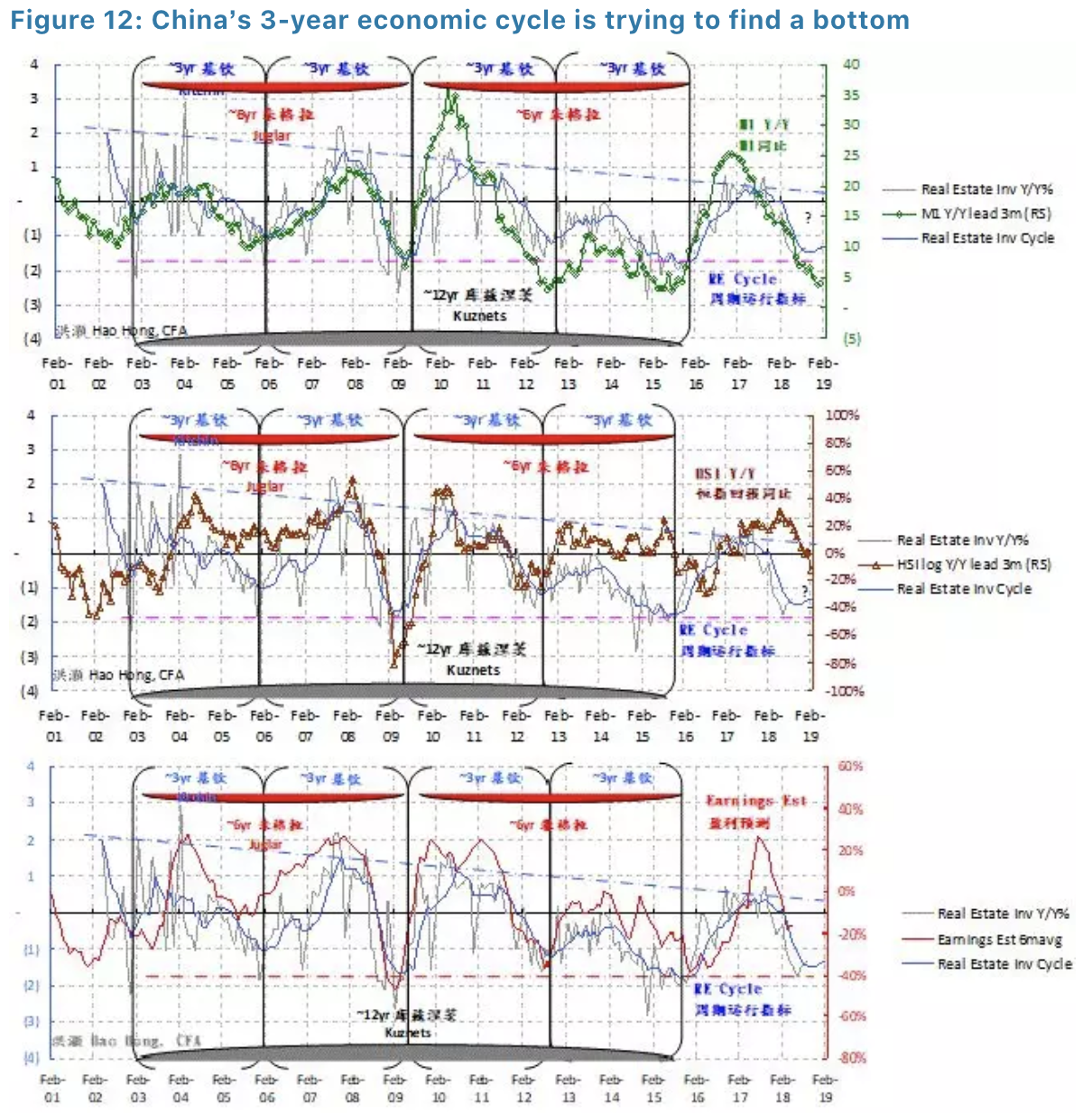
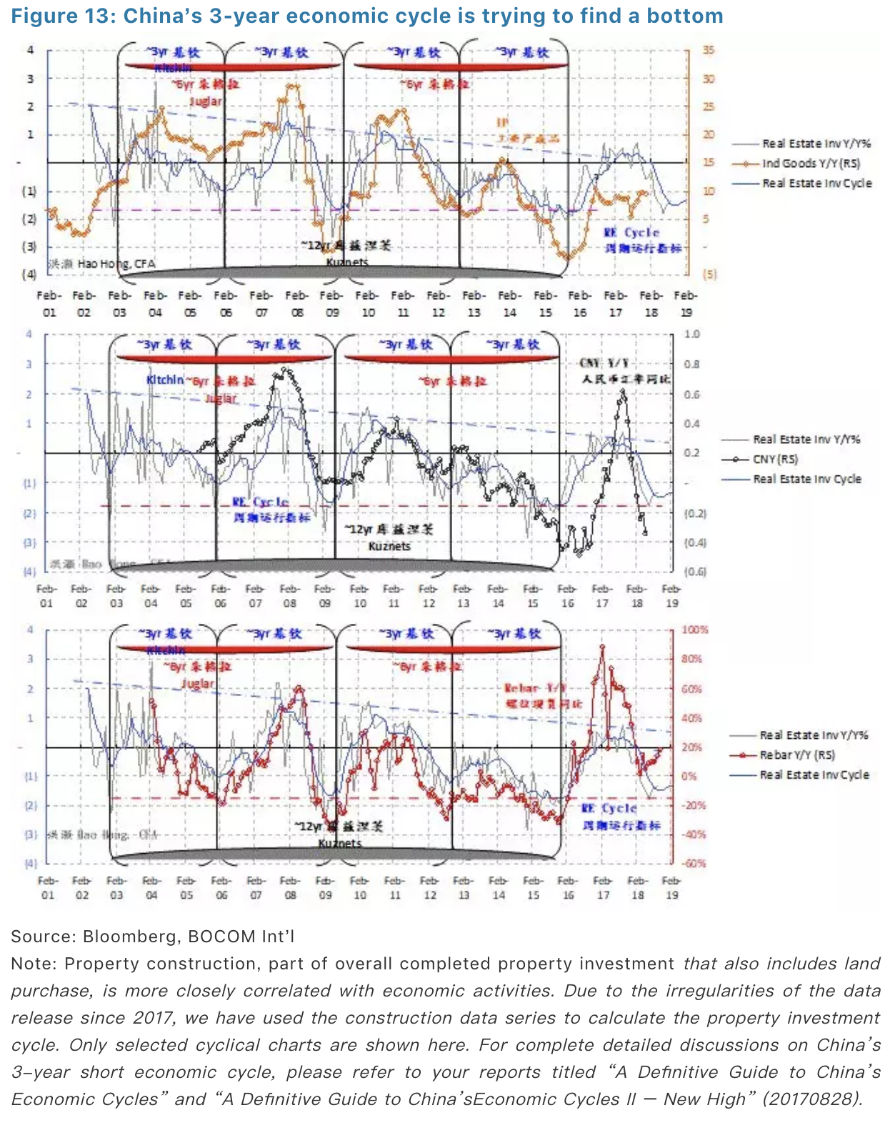
In our initial report on economic cycles with quantitative metrics titled “A Definitive Guide to China’s Economic Cycles” (20170323), we demonstrated the 3-year short cycle in the Chinese economy. We derive our 3-year investment cycle by measuring the deviation of the actual property investment growth data from its long-term trend. There have been by now almost five, very clearly defined 3-year cycles in China’s economy: 2003-2006, 2006-2009, 2009-2012, 2012-2015, and the last quarter of 2015 till now.
To verify the 3-year short cycle, we compare it with other macroeconomic variables in terms of both volume and price in the Chinese economy. Rebar price, interest rate level, industrial output, stock market indices and earnings forecasts, for instance. We have demonstrated that these variables are closely correlated (Not all comparisons are shown in this report. For detailed discussions on China’s short economic cycle, please refer to our report “A Definitive Guide to China’s Economic Cycles” on 20170323). That is, the 3-year short cycle can very well explain the movements in other Chinese macroeconomic variables (Figure 12).
Further, we note that in the past two decades of which period we have data, the trend of investment growth is falling, with lower highs and lower lows in each of the cycle sequentially. This is not difficult to fathom: China’s massive investment scale and increasing leverage are suppressing marginal investment return, and thus limiting the room for further productive investment.
We believe the duration of the 3-year cycle is related to China’s building construction process. For instance, to build a 30-storey residential building, the building completion time is around 9-12 months, water and electrical installation around 3 months, plus some more time for safety inspection and miscellaneous approvals. The total time to completion is around 1.5-2 years. Then the building inventory will take up to 1 year to clear, making the building inventory investment cycle to be around 3 years.
We note that the current 3-year short cycle that started from late 2015 to early 2016 has clearly peaked, and is trying to find a bottom, the momentum in the economic slowdown can intensify and turn even more palpable to consensus in the coming months (Figure 13). As such, while the market has reached its bottom range, its recovery will be hampered by overseas volatility – most notably from the US.
The short cycle in China
In our initial report on economic cycles with quantitative metrics titled “A Definitive Guide to China’s Economic Cycles” (20170323), we demonstrated the 3-year short cycle in the Chinese economy. We derive our 3-year investment cycle by measuring the deviation of the actual property investment growth data from its long-term trend. There have been by now almost five, very clearly defined 3-year cycles in China’s economy: 2003-2006, 2006-2009, 2009-2012, 2012-2015, and the last quarter of 2015 till now.
To verify the 3-year short cycle, we compare it with other macroeconomic variables in terms of both volume and price in the Chinese economy. Rebar price, interest rate level, industrial output, stock market indices and earnings forecasts, for instance. We have demonstrated that these variables are closely correlated (Not all comparisons are shown in this report. For detailed discussions on China’s short economic cycle, please refer to our report “A Definitive Guide to China’s Economic Cycles” on 20170323). That is, the 3-year short cycle can very well explain the movements in other Chinese macroeconomic variables (Figure 12).
Further, we note that in the past two decades of which period we have data, the trend of investment growth is falling, with lower highs and lower lows in each of the cycle sequentially. This is not difficult to fathom: China’s massive investment scale and increasing leverage are suppressing marginal investment return, and thus limiting the room for further productive investment.
We believe the duration of the 3-year cycle is related to China’s building construction process. For instance, to build a 30-storey residential building, the building completion time is around 9-12 months, water and electrical installation around 3 months, plus some more time for safety inspection and miscellaneous approvals. The total time to completion is around 1.5-2 years. Then the building inventory will take up to 1 year to clear, making the building inventory investment cycle to be around 3 years.
We note that the current 3-year short cycle that started from late 2015 to early 2016 has clearly peaked, and is trying to find a bottom, the momentum in the economic slowdown can intensify and turn even more palpable to consensus in the coming months (Figure 13). As such, while the market has reached its bottom range, its recovery will be hampered by overseas volatility – most notably from the US.
 FOUR: Market Outlook
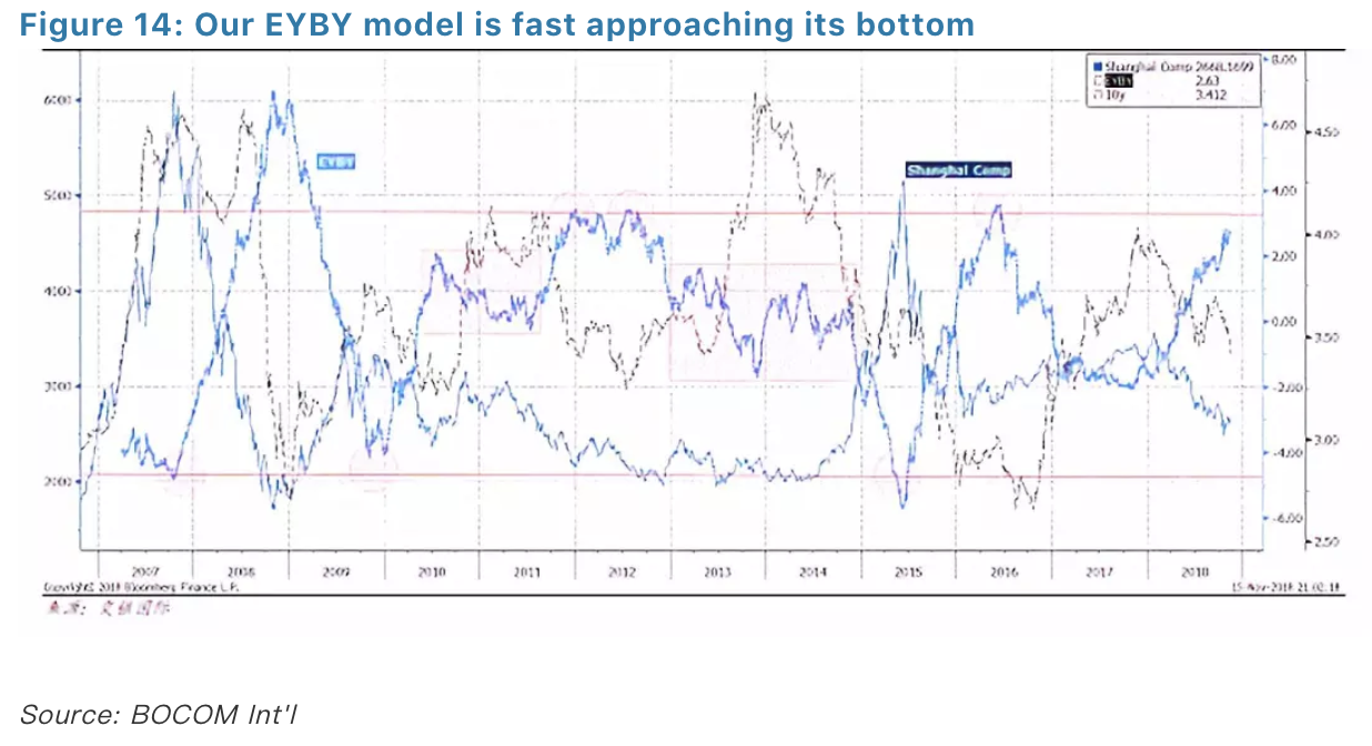
Bond yields should continue to fall heading into 2019; the Shanghai Composite has entered its bottom range as defined by our EYBY model (Figure 14) and our long-term allocation model. That said, we caution that the eventual bottom differs from the bottom range. An eventual bottom is the absolute lowest point, and can be only verified long after it occurs. The bottom range can be reasonably identified, but can be very volatile as traders regroup and expectations reshape. In sum, market bottom is a finite point on the index, while bottoming is a prolonged process in a range.
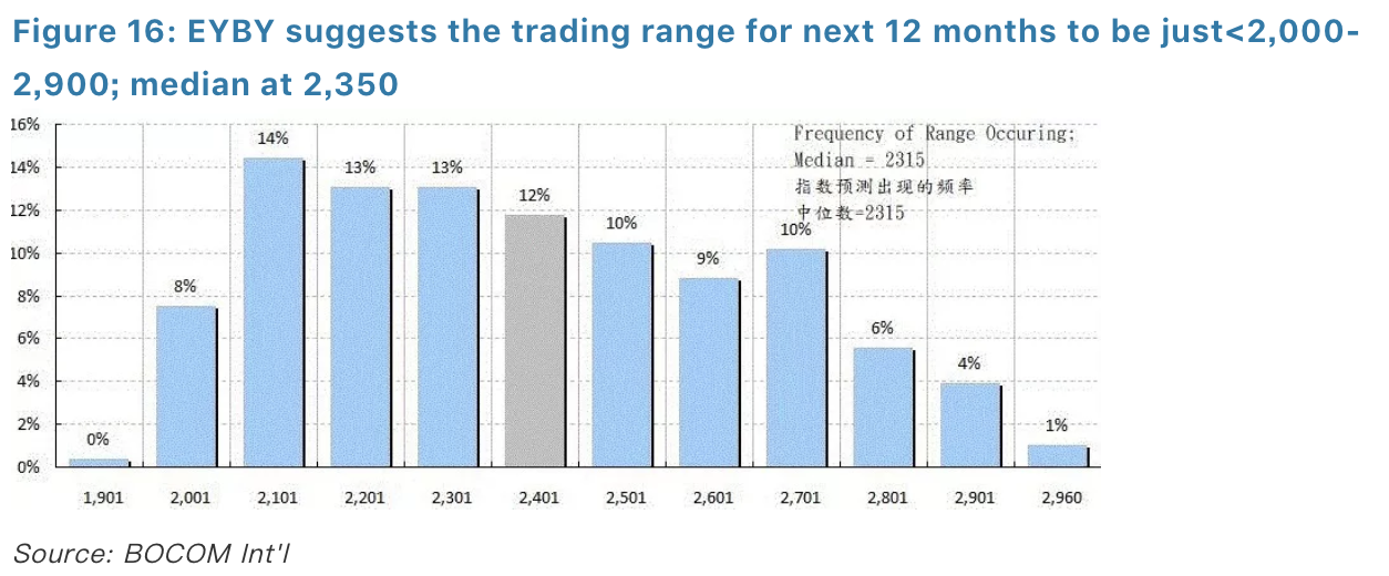
Our bond yield vs. earnings yield model (EYBY model hereafter) is suggesting a trading range of just under 2,000 to 2,900, with a median of around 2,350, for the Shanghai Composite in the coming 12 months. Further, the Shanghai Composite will spend at least six months trading above 2,350 in the next 12 months after the forecast (Figure 16).
FOUR: Market Outlook
Bond yields should continue to fall heading into 2019; the Shanghai Composite has entered its bottom range as defined by our EYBY model (Figure 14) and our long-term allocation model. That said, we caution that the eventual bottom differs from the bottom range. An eventual bottom is the absolute lowest point, and can be only verified long after it occurs. The bottom range can be reasonably identified, but can be very volatile as traders regroup and expectations reshape. In sum, market bottom is a finite point on the index, while bottoming is a prolonged process in a range.
Our bond yield vs. earnings yield model (EYBY model hereafter) is suggesting a trading range of just under 2,000 to 2,900, with a median of around 2,350, for the Shanghai Composite in the coming 12 months. Further, the Shanghai Composite will spend at least six months trading above 2,350 in the next 12 months after the forecast (Figure 16).
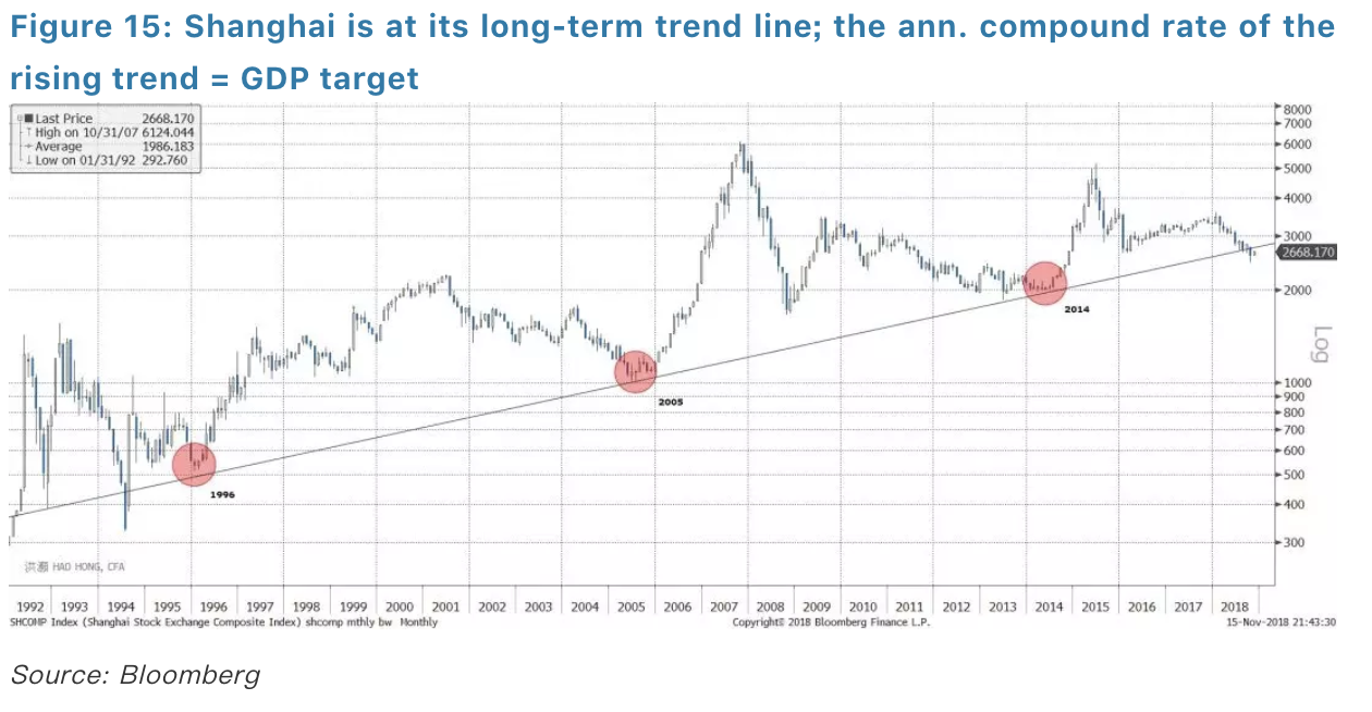
 In our report titled “The Market Bottom: When and Where” more than two years ago (20160604), we re-defined the market bottom as relative to a long-term economic growth rate. We showed that a log-linear relationship between the Shanghai Composite and the implicit GDP growth target implied by China’s Five-Year-Plan since 1986 (Figure 15). In this report two years ago, we posited that the theoretical market bottom should be around 2,450, should the historical relationship persist.
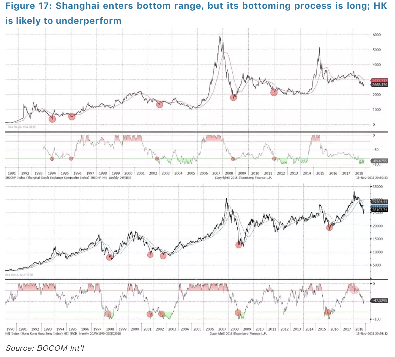
On 19 October 2018, the Shanghai Composite plunged to 2,449.197 before it rebounded. In the past two years, we have documented a mysterious force that has prevented the Shanghai Composite to arrive at its theoretical bottom, and have presented our findings to top policy makers (Figure 17). Recent public filings showed that the “National Team” had changed its way to support the market. With the prospects of a trade war and China’s ongoing structural reform, China’s long-term intrinsic growth rate could be revised down, leading the theoretical bottom to be lower than the 2,450 that we calculated more than two years ago. If so, it is consistent with our EYBY model result of 2,350 discussed above.
In our report titled “The Market Bottom: When and Where” more than two years ago (20160604), we re-defined the market bottom as relative to a long-term economic growth rate. We showed that a log-linear relationship between the Shanghai Composite and the implicit GDP growth target implied by China’s Five-Year-Plan since 1986 (Figure 15). In this report two years ago, we posited that the theoretical market bottom should be around 2,450, should the historical relationship persist.
On 19 October 2018, the Shanghai Composite plunged to 2,449.197 before it rebounded. In the past two years, we have documented a mysterious force that has prevented the Shanghai Composite to arrive at its theoretical bottom, and have presented our findings to top policy makers (Figure 17). Recent public filings showed that the “National Team” had changed its way to support the market. With the prospects of a trade war and China’s ongoing structural reform, China’s long-term intrinsic growth rate could be revised down, leading the theoretical bottom to be lower than the 2,450 that we calculated more than two years ago. If so, it is consistent with our EYBY model result of 2,350 discussed above.
 Our EYBY model has helped us pinpoint the bottom of China’s stock market after mid-2014, as well as the peak of the bubble in June 2015. The model has also helped us negotiate the rough waters after the bubble burst.
The model forecast of trading range for the 12 months after its publication was 2,800 – 3,800, compared with the actual trading range of 2,450-3,600. Clearly, we underestimated the impact from the trade war. Yet, our forecast of the lower range was still the most pessimistic on the street at the time of its publication. Further, the model forecasted that the Shanghai Composite would spend more than six months below 3,200 in the 12 months after the forecast. The actual result is that on only 100 trading days out of the 260 trading days since its publication the Shanghai Composite managed to stay above 3,200.
In December 2014 when we were preparing the 2015 outlook, the model forecasted that a market bubble was looming, but the year of 2015 should finish at not much higher than 3,400. The Shanghai Composite finished at ~3,300 one trading day after the last trading day in 2015; in December 2015 when we were preparing the 2016 outlook, the model forecasted that the trading range for 2016 should be 2,500-3,300, versus the final actual range of 2,638-3,301; in December 2016 when we prepared the 2017 outlook, the model forecasted in 2017 the Shanghai Composite should spend at least eight months below 3,300. And the composite didn’t first close above 3,300 until 25 August 2017 – slightly more than eight months after our original forecast in early December 2016.
The pace of how fast equity valuation can heal relative to the fall in bond yield determines how far the stock indices can rise, as funds rotate from bonds to equities for value. As liquidity should continue to loosen, bond yield should continue to fall.
Our EYBY model has helped us pinpoint the bottom of China’s stock market after mid-2014, as well as the peak of the bubble in June 2015. The model has also helped us negotiate the rough waters after the bubble burst.
The model forecast of trading range for the 12 months after its publication was 2,800 – 3,800, compared with the actual trading range of 2,450-3,600. Clearly, we underestimated the impact from the trade war. Yet, our forecast of the lower range was still the most pessimistic on the street at the time of its publication. Further, the model forecasted that the Shanghai Composite would spend more than six months below 3,200 in the 12 months after the forecast. The actual result is that on only 100 trading days out of the 260 trading days since its publication the Shanghai Composite managed to stay above 3,200.
In December 2014 when we were preparing the 2015 outlook, the model forecasted that a market bubble was looming, but the year of 2015 should finish at not much higher than 3,400. The Shanghai Composite finished at ~3,300 one trading day after the last trading day in 2015; in December 2015 when we were preparing the 2016 outlook, the model forecasted that the trading range for 2016 should be 2,500-3,300, versus the final actual range of 2,638-3,301; in December 2016 when we prepared the 2017 outlook, the model forecasted in 2017 the Shanghai Composite should spend at least eight months below 3,300. And the composite didn’t first close above 3,300 until 25 August 2017 – slightly more than eight months after our original forecast in early December 2016.
The pace of how fast equity valuation can heal relative to the fall in bond yield determines how far the stock indices can rise, as funds rotate from bonds to equities for value. As liquidity should continue to loosen, bond yield should continue to fall.