Hong Hao: Outlook 2020: Going the Distance
2019-11-14 IMI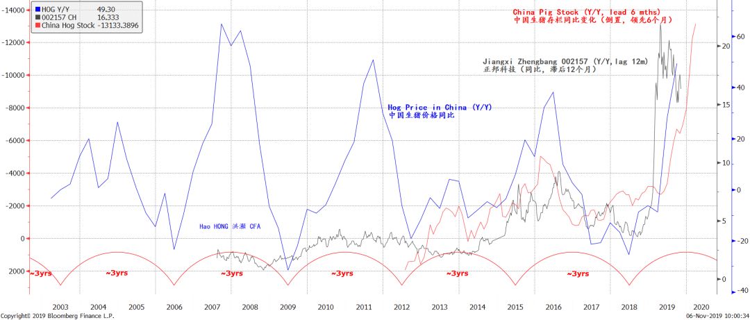 Source: Bloomberg, BOCOM Int'l
The shortfall in pig stock tends to lead hog price inflation by about 6 months historically (Figure 1). Since the second half of 2018, the pig stock in China has been devastated by the severe outbreak of the African Swine Fever. The country’s pig stock has now fallen by ~130 million year on year, which is close to the entire pig population of ~150 million in the EU, and almost double the size of that of the US.
The intensity of the current hog price inflation in China rivals the previous peaks in history (Figure 1). However, the reduction of pig stock in China is unprecedented, and is likely to induce a super hog cycle unseen before. The hog cycle in China tends to run for approximately three years, and its wave length has been largely consistent with that of China’s short economic cycle. Given the severe pig shortage, this hog cycle can run substantially higher than previous cycles. It will hamper the choice of monetary policy in the near term, lessening the chance and the depth of any potential rate cut.
Figure 2: The effect of RRR cuts on monetary condition has a long lag, especially when inflation is high
Source: Bloomberg, BOCOM Int'l
The shortfall in pig stock tends to lead hog price inflation by about 6 months historically (Figure 1). Since the second half of 2018, the pig stock in China has been devastated by the severe outbreak of the African Swine Fever. The country’s pig stock has now fallen by ~130 million year on year, which is close to the entire pig population of ~150 million in the EU, and almost double the size of that of the US.
The intensity of the current hog price inflation in China rivals the previous peaks in history (Figure 1). However, the reduction of pig stock in China is unprecedented, and is likely to induce a super hog cycle unseen before. The hog cycle in China tends to run for approximately three years, and its wave length has been largely consistent with that of China’s short economic cycle. Given the severe pig shortage, this hog cycle can run substantially higher than previous cycles. It will hamper the choice of monetary policy in the near term, lessening the chance and the depth of any potential rate cut.
Figure 2: The effect of RRR cuts on monetary condition has a long lag, especially when inflation is high
 Source: Bloomberg, BOCOM Int'l
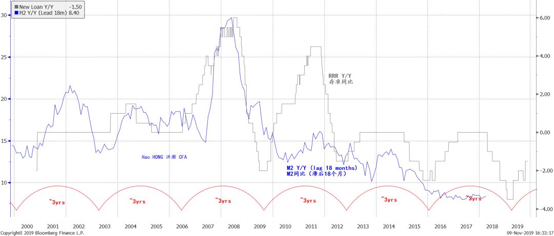
China’s RRR cuts have so far failed to generate sustainable lending growth. This is because RRR cuts tend to influence monetary conditions with a lag of up to 18 months (Figure 2). The change in RRR also runs with a cycle of roughly three years. In early 2019, we have seen this long leading indicator bottoming out. As such, easing liquidity conditions will come eventually, although we must wait a little while longer - till the inflation pressure starts to dissipate.
Even though inflation pressure driven by China’s super hog cycle is likely to mount in the coming months, we believe the longer-term trend for inflation is still declining. The PBoC’s monetary objective has remained surprisingly neutral and restrained, with a stated policy objective to keep M2 growth consistent with nominal GDP growth.
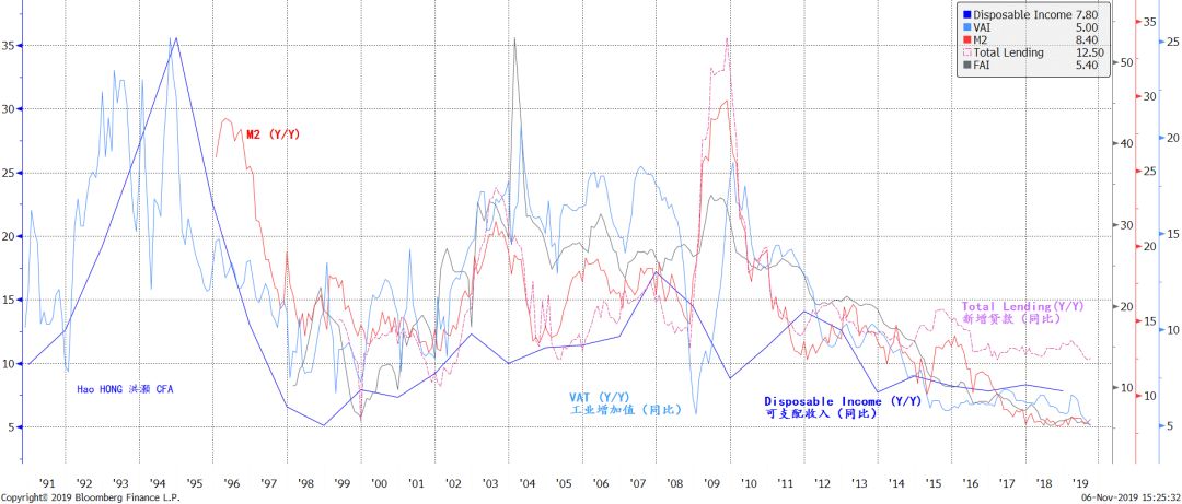
Money supply growth determines lending, investment, economic growth, and ultimately the growth of disposable income. If the longer-term trend of M2 growth is falling, so will disposable income growth (Figure 3). As such, as long as productivity gain, which is increasingly from the exponential growth of computing power, rises faster than income, as it has been, the longer-term outlook for inflation should be declining as well.
Figure 3: Falling money supply, investment, growth and hence income curtail longer-term inflation
Source: Bloomberg, BOCOM Int'l
China’s RRR cuts have so far failed to generate sustainable lending growth. This is because RRR cuts tend to influence monetary conditions with a lag of up to 18 months (Figure 2). The change in RRR also runs with a cycle of roughly three years. In early 2019, we have seen this long leading indicator bottoming out. As such, easing liquidity conditions will come eventually, although we must wait a little while longer - till the inflation pressure starts to dissipate.
Even though inflation pressure driven by China’s super hog cycle is likely to mount in the coming months, we believe the longer-term trend for inflation is still declining. The PBoC’s monetary objective has remained surprisingly neutral and restrained, with a stated policy objective to keep M2 growth consistent with nominal GDP growth.
Money supply growth determines lending, investment, economic growth, and ultimately the growth of disposable income. If the longer-term trend of M2 growth is falling, so will disposable income growth (Figure 3). As such, as long as productivity gain, which is increasingly from the exponential growth of computing power, rises faster than income, as it has been, the longer-term outlook for inflation should be declining as well.
Figure 3: Falling money supply, investment, growth and hence income curtail longer-term inflation
 Source: Bloomberg, BOCOM Int'l estimates
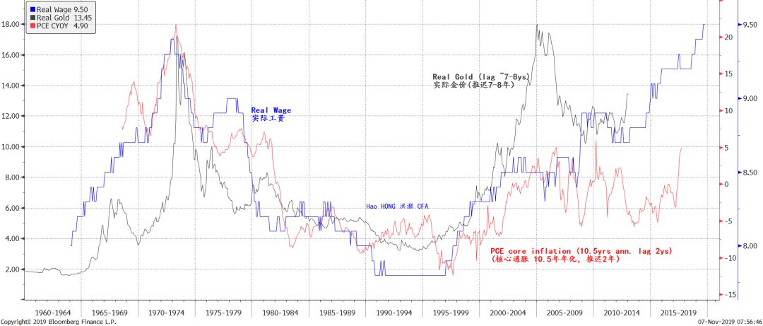
In the US, we find that inflation pressure is slowly building as well. We note that the real wage in the US has returned to its previous highs seen in early 1970s. If we compare the US real wage with US PCE core inflation annualized on a 10.5-year basis with a roughly two-year lag, we can see a clear correlation, and a trend of rising US core inflation (Figure 4; Note that the 10.5-year basis for our analysis is consistent with the wave length of an intermediate economic cycle consisting of three 3.5-year short cycles.
There is also close correlation between real wage in the US and the inflation-adjusted gold price, with a lag of roughly seven years (the wave length of an intermediate cycle consisting of two 3.5-year cycles). In short, real wage growth can forecast the direction of US inflation and gold price, with a substantial lead (Figure 4).
Figure 4: US core inflation pressure is slowly accumulating, as US employment reaches cycle peak
Source: Bloomberg, BOCOM Int'l estimates
In the US, we find that inflation pressure is slowly building as well. We note that the real wage in the US has returned to its previous highs seen in early 1970s. If we compare the US real wage with US PCE core inflation annualized on a 10.5-year basis with a roughly two-year lag, we can see a clear correlation, and a trend of rising US core inflation (Figure 4; Note that the 10.5-year basis for our analysis is consistent with the wave length of an intermediate economic cycle consisting of three 3.5-year short cycles.
There is also close correlation between real wage in the US and the inflation-adjusted gold price, with a lag of roughly seven years (the wave length of an intermediate cycle consisting of two 3.5-year cycles). In short, real wage growth can forecast the direction of US inflation and gold price, with a substantial lead (Figure 4).
Figure 4: US core inflation pressure is slowly accumulating, as US employment reaches cycle peak
 Source: Bloomberg, BOCOM Int'l estimates
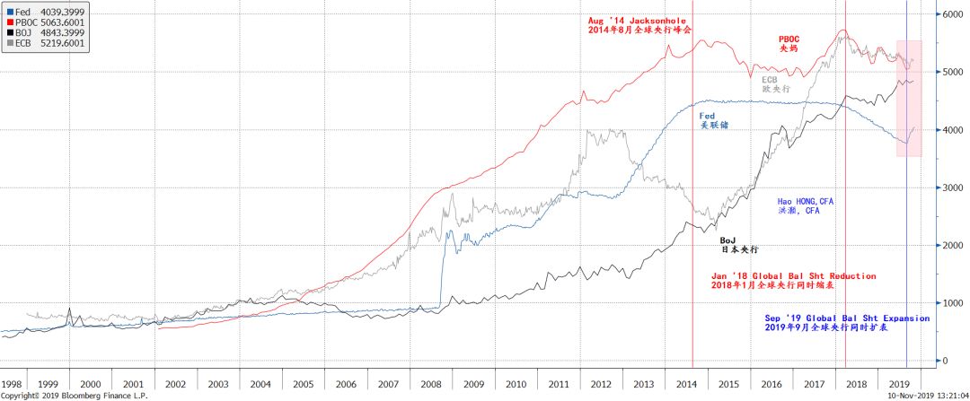
If inflationary pressure in the US is indeed slowly rising, as suggested by Figure 4, and the short economic cycle is healing (to be discussed later), the Fed’s path to rate cuts as anticipated by the market could be altered. But the Fed’s plan to re-expand its balance sheet together with the other major global central banks is likely to be intact (Figure 5).
Figure 5: Global central banks are re-expanding their balance sheets
Source: Bloomberg, BOCOM Int'l estimates
If inflationary pressure in the US is indeed slowly rising, as suggested by Figure 4, and the short economic cycle is healing (to be discussed later), the Fed’s path to rate cuts as anticipated by the market could be altered. But the Fed’s plan to re-expand its balance sheet together with the other major global central banks is likely to be intact (Figure 5).
Figure 5: Global central banks are re-expanding their balance sheets
 Source: Bloomberg, BOCOM Int'l estimates
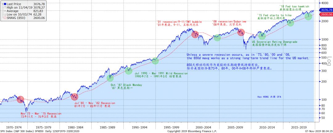
Such a discrepancy in the market’s expectation of rate cuts, though in part being gradually reflected in the Fed funds futures, can induce disruption in the stock market in 2020. That said, without recession, the rising trend in the US market will persist, with the 850-day moving average being the secular rising trend line (Figure 6). The last leg up will likely squeeze many doubters of the US market’s strength, burying a lot of shorts and then the longs after the eventual market peak.
Figure 6: 850-day mavg is a secular rising trend line for SPX; only severe US recessions could puncture it
Source: Bloomberg, BOCOM Int'l estimates
Such a discrepancy in the market’s expectation of rate cuts, though in part being gradually reflected in the Fed funds futures, can induce disruption in the stock market in 2020. That said, without recession, the rising trend in the US market will persist, with the 850-day moving average being the secular rising trend line (Figure 6). The last leg up will likely squeeze many doubters of the US market’s strength, burying a lot of shorts and then the longs after the eventual market peak.
Figure 6: 850-day mavg is a secular rising trend line for SPX; only severe US recessions could puncture it
 Source: Bloomberg, BOCOM Int'l estimates
China’s Leading Economic Cycle Indicator to Moderate
In our initial report on economic cycles with quantitative metrics titled “A Definitive Guide to China’s Economic Cycles” (20170324), we demonstrated the 3-year short cycle in the Chinese economy. We derive our 3-year investment cycle by measuring the deviation of the actual property investment growth data from its long-term trend. There have been by now almost six, very clearly-defined 3-year cycles in China’s economy: 2003-2006, 2006-2009, 2009-2012, 2012-2015, and the last quarter of 2015/early 2016 till the end of 2018.
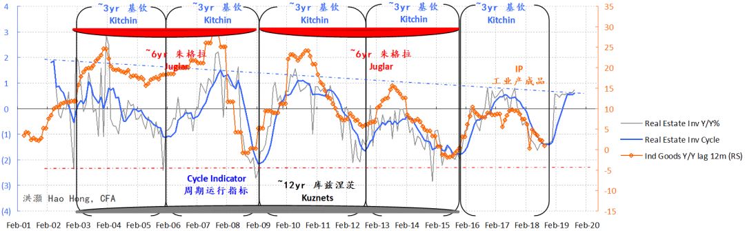
To verify the 3-year short cycle, we compare it with other macroeconomic variables in terms of both volume and price in the Chinese economy. Rebar price, interest rate level, industrial output, stock market indices and earnings forecasts, for instance. We have demonstrated that these variables are closely correlated (not all comparisons are shown in this report; for detailed discussions on China’s short economic cycle, please refer to our report “A Definitive Guide to China’s Economic Cycles” on 20170324). That is, the 3-year short cycle can very well explain the movements in many other Chinese macroeconomic variables (Figure 7).
Further, we note that in the past two decades of which period we have data, the trend of investment growth is falling, with lower highs and lower lows in each of the cycle sequentially. This is not difficult to fathom: China’s massive investment scale and increasing leverage are suppressing marginal investment return, and thus limiting the room for further productive investment.
We believe the duration of the 3-year cycle is related to China’s building construction process. For instance, to build a 30-storey residential building, the building completion time is around 9-12 months, water and electrical installation around 3 months, plus some more time for safety inspection and miscellaneous approvals. The total time to completion is around 1.5-2 years. Then, the building inventory will take up to 1 year to clear, making the building inventory investment cycle of around 3 years.
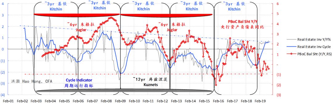
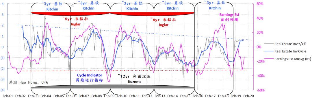
We note that the current 3-year short cycle that started from late 2018 to early 2019 is peaking, driven by moderating property investment growth after double-digit growth in 2019. That said, as our cycle indicator is a leading measure, the momentum in nominal economic variables driven by surging inflation pressure can still show persistency in the coming months (Figure 7).
Investors should not be fooled by these nominal and lagging improvements that have been well foretold by our cycle leading indicator and thus are already priced in. Unless the nominal improvements beat market expectations significantly, stock prices will not respond. In general, in a slowing environment with persistent inflation pressure in the coming months, investors will find it difficult to commit capital to stocks or bonds.
Figure 7: China’s leading economic cycle indicator will likely moderate in the coming months, but China leads
Source: Bloomberg, BOCOM Int'l estimates
China’s Leading Economic Cycle Indicator to Moderate
In our initial report on economic cycles with quantitative metrics titled “A Definitive Guide to China’s Economic Cycles” (20170324), we demonstrated the 3-year short cycle in the Chinese economy. We derive our 3-year investment cycle by measuring the deviation of the actual property investment growth data from its long-term trend. There have been by now almost six, very clearly-defined 3-year cycles in China’s economy: 2003-2006, 2006-2009, 2009-2012, 2012-2015, and the last quarter of 2015/early 2016 till the end of 2018.
To verify the 3-year short cycle, we compare it with other macroeconomic variables in terms of both volume and price in the Chinese economy. Rebar price, interest rate level, industrial output, stock market indices and earnings forecasts, for instance. We have demonstrated that these variables are closely correlated (not all comparisons are shown in this report; for detailed discussions on China’s short economic cycle, please refer to our report “A Definitive Guide to China’s Economic Cycles” on 20170324). That is, the 3-year short cycle can very well explain the movements in many other Chinese macroeconomic variables (Figure 7).
Further, we note that in the past two decades of which period we have data, the trend of investment growth is falling, with lower highs and lower lows in each of the cycle sequentially. This is not difficult to fathom: China’s massive investment scale and increasing leverage are suppressing marginal investment return, and thus limiting the room for further productive investment.
We believe the duration of the 3-year cycle is related to China’s building construction process. For instance, to build a 30-storey residential building, the building completion time is around 9-12 months, water and electrical installation around 3 months, plus some more time for safety inspection and miscellaneous approvals. The total time to completion is around 1.5-2 years. Then, the building inventory will take up to 1 year to clear, making the building inventory investment cycle of around 3 years.
We note that the current 3-year short cycle that started from late 2018 to early 2019 is peaking, driven by moderating property investment growth after double-digit growth in 2019. That said, as our cycle indicator is a leading measure, the momentum in nominal economic variables driven by surging inflation pressure can still show persistency in the coming months (Figure 7).
Investors should not be fooled by these nominal and lagging improvements that have been well foretold by our cycle leading indicator and thus are already priced in. Unless the nominal improvements beat market expectations significantly, stock prices will not respond. In general, in a slowing environment with persistent inflation pressure in the coming months, investors will find it difficult to commit capital to stocks or bonds.
Figure 7: China’s leading economic cycle indicator will likely moderate in the coming months, but China leads
 Source: BOCOM Int'l estimates
The Global Cycle is Healing
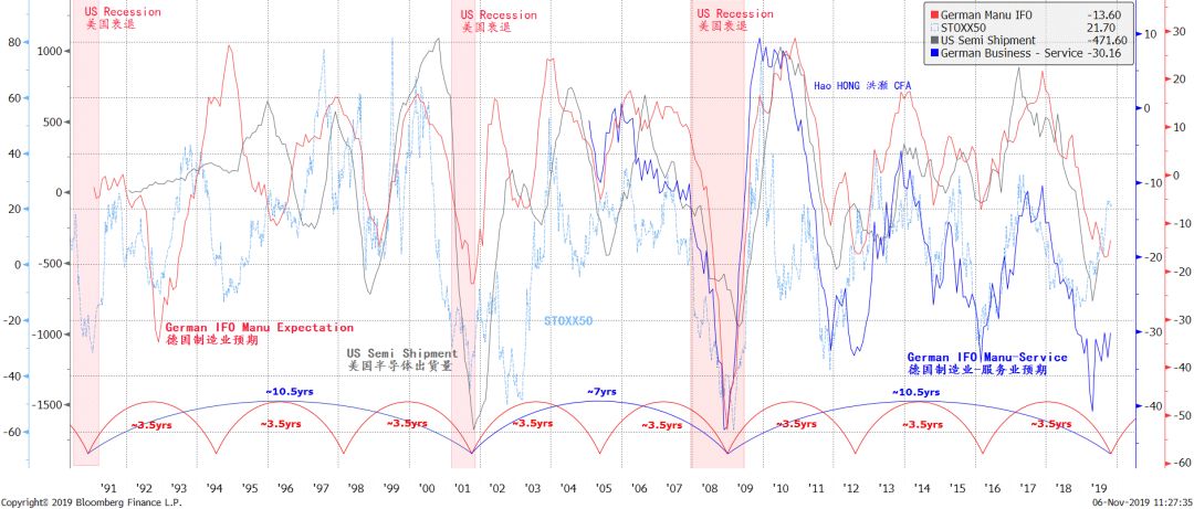
Globally, the short economic cycle appears to be bottoming out in both EU and the US (Figure 8). The short economic cycle in the EU and the US, as approximated by German manufacturing IFO, US semi shipment growth and EPS growth, operates with a wave length of roughly 3.5 years (“The Colliding Cycles of the US and China” 20180903 and “A Definitive Guide to Forecasting China Market” 20190920). Its length is largely consistent with China’s short economic cycle, but runs with a lag.
Figure 8: The short economic cycle in both the EU and the US is healing
Source: BOCOM Int'l estimates
The Global Cycle is Healing
Globally, the short economic cycle appears to be bottoming out in both EU and the US (Figure 8). The short economic cycle in the EU and the US, as approximated by German manufacturing IFO, US semi shipment growth and EPS growth, operates with a wave length of roughly 3.5 years (“The Colliding Cycles of the US and China” 20180903 and “A Definitive Guide to Forecasting China Market” 20190920). Its length is largely consistent with China’s short economic cycle, but runs with a lag.
Figure 8: The short economic cycle in both the EU and the US is healing
 Source: Bloomberg, BOCOM Int'l estimates
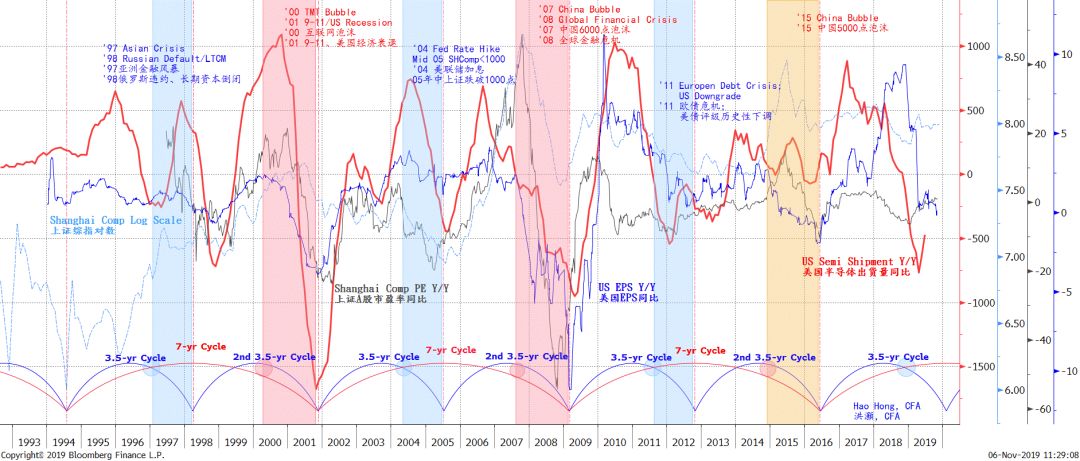
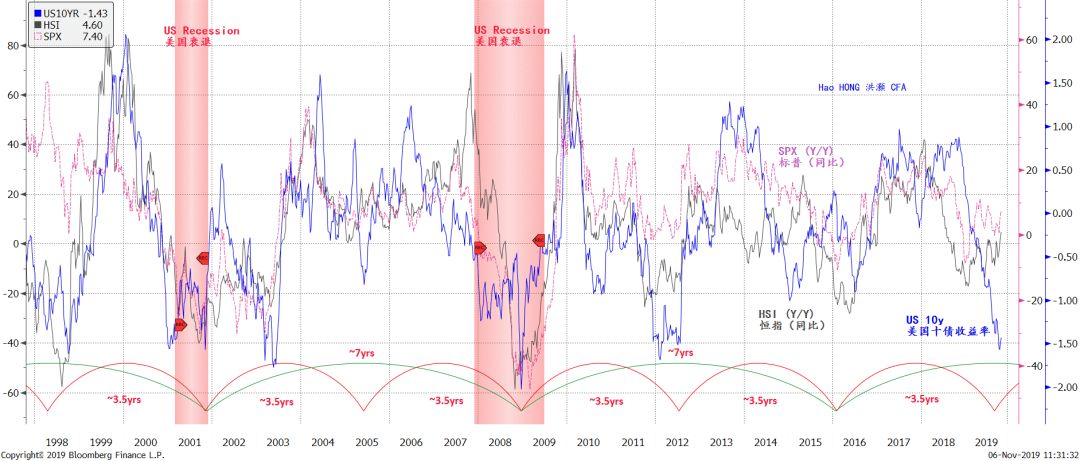
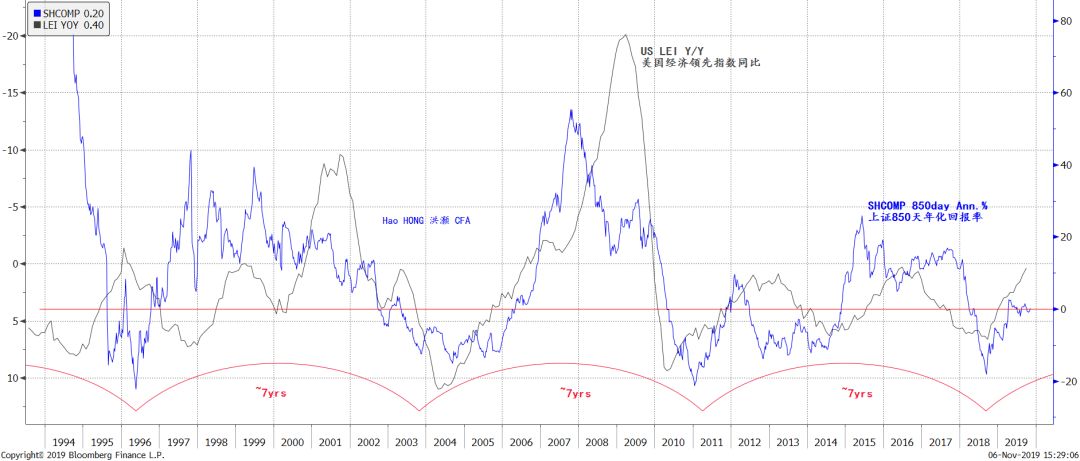
Meanwhile, the US 10-year yield is bottoming out from a very depressed level that historically augured economic recession or market turmoil, as in 2001/02, 2008, 2012 and 2015/16 (Figure 9). Yield curve re-steepening can alleviate the recession fears. As China’s cycle of stock market return continues to recover from the bottom of a 7-year cycle seen in late 2018 and early 2019, the US Leading Economic Indicator is reflating concurrently (Figure 10). Yet, the market remains skeptical about the health of the US economy, despite the help from the Fed.
Figure 9: The global cycle is healing (cont’d)
Source: Bloomberg, BOCOM Int'l estimates
Meanwhile, the US 10-year yield is bottoming out from a very depressed level that historically augured economic recession or market turmoil, as in 2001/02, 2008, 2012 and 2015/16 (Figure 9). Yield curve re-steepening can alleviate the recession fears. As China’s cycle of stock market return continues to recover from the bottom of a 7-year cycle seen in late 2018 and early 2019, the US Leading Economic Indicator is reflating concurrently (Figure 10). Yet, the market remains skeptical about the health of the US economy, despite the help from the Fed.
Figure 9: The global cycle is healing (cont’d)
 Source: Bloomberg, BOCOM Int'l estimates
Figure 10: China’s cycle is leading the global cycle
Source: Bloomberg, BOCOM Int'l estimates
Figure 10: China’s cycle is leading the global cycle
 Source: Bloomberg, BOCOM Int'l estimates
As such, the strength of the US market rebound can surprise many bears – as the final short squeezes prior to the eventual market downturn always do. In 2020, we would also watch the US election closely. It will be a showdown between the capitalists and the socialists. For now, it is difficult to fight the global central banks that are re-expanding their balance sheets simultaneously.
A History of US Investment Return and its Implications
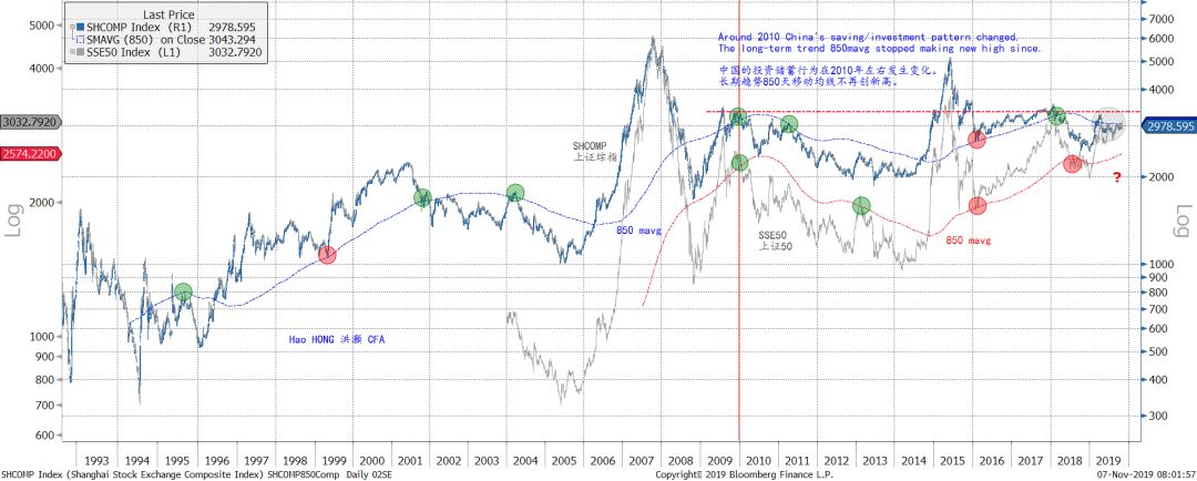
In our previous report titled “A Definitive Guide to Forecasting China Market” (20190920), we discussed that 2010 is the watershed year in asset allocation in China. Current account surplus to GDP ratio, money supply growth and FAI growth all peaked around 2010 and have declined ever since then.
Consequently, the 850-day moving average of the Shanghai Composite has not made any new high above ~3,200 since 2010. China’s stock market has turned into a zero-sum game since then. Even the bubble in 2015, though significantly breaking through 3,200, did not take the moving average to new higher levels.
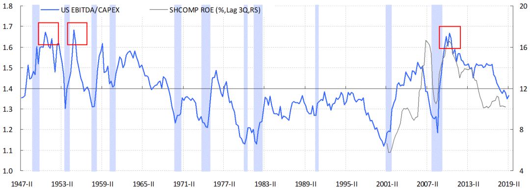
Globally, we notice a similar development. Using the US Flow of Funds data, we calculate the EBITDA-to-Capex ratio in the US economy, and use this ratio as a proxy for investment return in the US. We find that investment return in the US has also peaked around 2010, and has been falling ever since, albeit not to the recessionary levels seen during the recessions since 1970s. As our analysis shows, the ROE of the Shanghai Composite and the US investment return are closely related (Figure 11).
Figure 11: US investment return and China’s ROE have both been falling since 2010/11
Source: Bloomberg, BOCOM Int'l estimates
As such, the strength of the US market rebound can surprise many bears – as the final short squeezes prior to the eventual market downturn always do. In 2020, we would also watch the US election closely. It will be a showdown between the capitalists and the socialists. For now, it is difficult to fight the global central banks that are re-expanding their balance sheets simultaneously.
A History of US Investment Return and its Implications
In our previous report titled “A Definitive Guide to Forecasting China Market” (20190920), we discussed that 2010 is the watershed year in asset allocation in China. Current account surplus to GDP ratio, money supply growth and FAI growth all peaked around 2010 and have declined ever since then.
Consequently, the 850-day moving average of the Shanghai Composite has not made any new high above ~3,200 since 2010. China’s stock market has turned into a zero-sum game since then. Even the bubble in 2015, though significantly breaking through 3,200, did not take the moving average to new higher levels.
Globally, we notice a similar development. Using the US Flow of Funds data, we calculate the EBITDA-to-Capex ratio in the US economy, and use this ratio as a proxy for investment return in the US. We find that investment return in the US has also peaked around 2010, and has been falling ever since, albeit not to the recessionary levels seen during the recessions since 1970s. As our analysis shows, the ROE of the Shanghai Composite and the US investment return are closely related (Figure 11).
Figure 11: US investment return and China’s ROE have both been falling since 2010/11
 Source: Bloomberg, BOCOM Int'l estimates
It is difficult to dismiss this correlation as mere coincidence, given the inter-dependence between the US and Chinese economy. Historically, China produces and US consumes. The US spends and China saves. The accumulations of positions for FX purchases, or the PBoC’s sterilization operations, have been the most important source of liquidity for China.
Since the Great Recession in 2008, however, the US has been disenchanted by gloomy outlook and has been saving hard. This change in saving habit can be seen in the rising national savings rate in the US, concurrent with the rising current account surplus. The savings glut depresses investment return, and affects the investment outlook for the US public, who in turn saves even harder. Consequently, investment return in the US continues to fall, as seen in Figure 11.
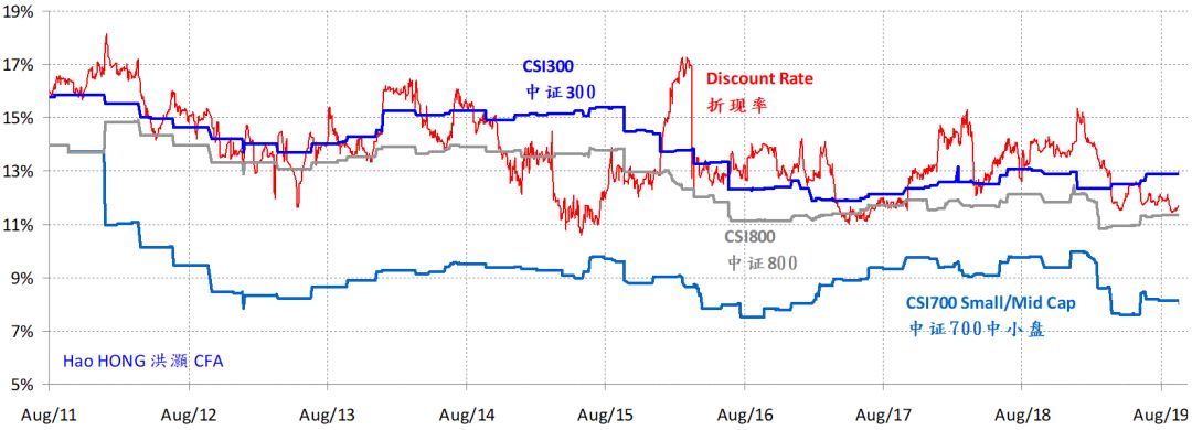
Meanwhile, in China, because the foreign source of liquidity is dwindling, Chinese growth that used to be driven by credits starts to slow, and hence ROE. Indeed, we observe falling ROE across all market caps in China since 2010. And the ROE of mid/small caps is falling much faster than that of large caps, and is now well below the equity discount rate. That is, the mid/small caps are now earning negative economic return, while the large caps are managing to stay above the general equity discount rate (Figure 12).
Figure 12: Return in China has been falling; divergence between large and mid/small caps
Source: Bloomberg, BOCOM Int'l estimates
It is difficult to dismiss this correlation as mere coincidence, given the inter-dependence between the US and Chinese economy. Historically, China produces and US consumes. The US spends and China saves. The accumulations of positions for FX purchases, or the PBoC’s sterilization operations, have been the most important source of liquidity for China.
Since the Great Recession in 2008, however, the US has been disenchanted by gloomy outlook and has been saving hard. This change in saving habit can be seen in the rising national savings rate in the US, concurrent with the rising current account surplus. The savings glut depresses investment return, and affects the investment outlook for the US public, who in turn saves even harder. Consequently, investment return in the US continues to fall, as seen in Figure 11.
Meanwhile, in China, because the foreign source of liquidity is dwindling, Chinese growth that used to be driven by credits starts to slow, and hence ROE. Indeed, we observe falling ROE across all market caps in China since 2010. And the ROE of mid/small caps is falling much faster than that of large caps, and is now well below the equity discount rate. That is, the mid/small caps are now earning negative economic return, while the large caps are managing to stay above the general equity discount rate (Figure 12).
Figure 12: Return in China has been falling; divergence between large and mid/small caps
 Source: Bloomberg, BOCOM Int'l estimates
Such diverging ROE between large and mid/small caps explains the “leader effect” in recent years, as the leading companies in their respective industries substantially outperform the rest of the industry. Similar market performance as a result of industry concentration is also seen in the US.
The relationship of the large-cap index with its 850-day moving average contrasts starkly with that of the small/mid-cap index. For the large-cap indices represented by the SSE50 or CSI300, they stay well above the 850-day moving average. The average has been acting as a strong support for the underlying rising trend of the large caps. On the contrary, the moving average is acting as a strong resistance for the small/mid-cap indices represented by CSI700, and the overall broad market index of the Shanghai Composite (Figure 13).
As such, without a major paradigm shift for the small/mid-caps, we should expect continuing relative outperformance from the large caps. Even the targeted policies to help out the small businesses may not be able to turn the tables for now.
Figure 13: The 850-day mavg is a strong resistance for the Shanghai Comp, but a strong support for SSE50
Source: Bloomberg, BOCOM Int'l estimates
Such diverging ROE between large and mid/small caps explains the “leader effect” in recent years, as the leading companies in their respective industries substantially outperform the rest of the industry. Similar market performance as a result of industry concentration is also seen in the US.
The relationship of the large-cap index with its 850-day moving average contrasts starkly with that of the small/mid-cap index. For the large-cap indices represented by the SSE50 or CSI300, they stay well above the 850-day moving average. The average has been acting as a strong support for the underlying rising trend of the large caps. On the contrary, the moving average is acting as a strong resistance for the small/mid-cap indices represented by CSI700, and the overall broad market index of the Shanghai Composite (Figure 13).
As such, without a major paradigm shift for the small/mid-caps, we should expect continuing relative outperformance from the large caps. Even the targeted policies to help out the small businesses may not be able to turn the tables for now.
Figure 13: The 850-day mavg is a strong resistance for the Shanghai Comp, but a strong support for SSE50
 Source: Bloomberg, BOCOM Int'l estimates
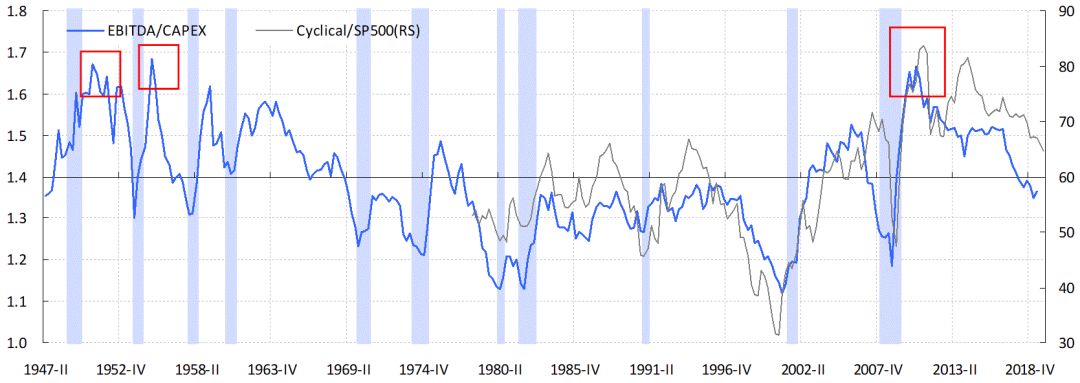
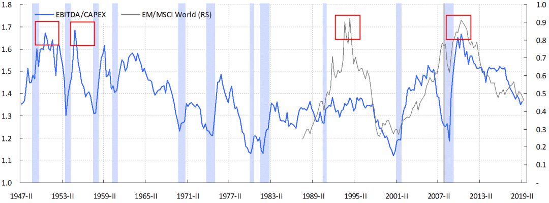
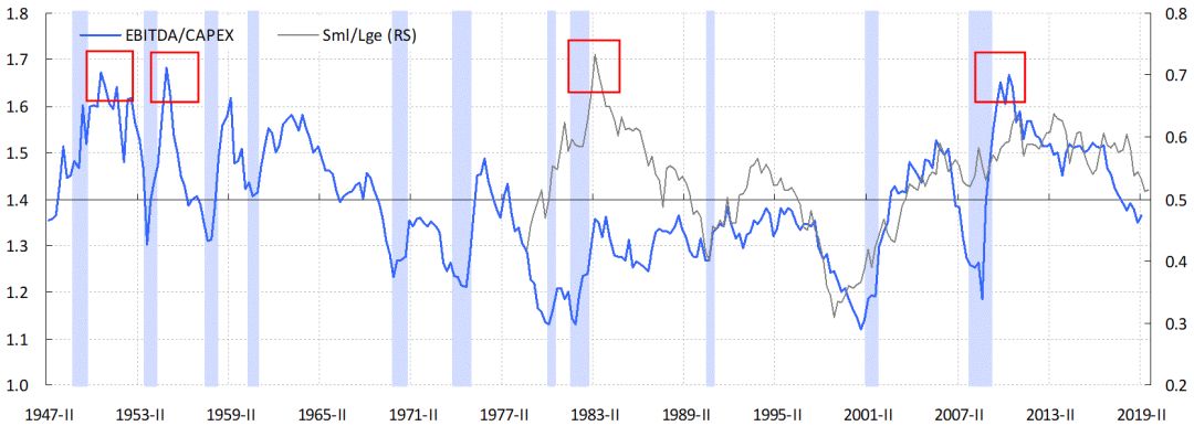
The US investment return, as measured by the ratio between EBITDA and Capex, is also an excellent proxy for the global investment environment. Our analysis finds the US investment return highly correlated with the relative performance of global cyclicals vs. defensive, EM vs. the world, and small vs. large caps (Figure 14).
Since around 2010, cyclicals, EM and small caps have been underperforming. That said, even though by now the underperformance has persisted for years, and may be prone to a technical rebound in the near term, it is unlikely to have run its course. Ever falling interest rates, and the prospect of negative interest rate, will prompt people to save harder, as suggested by the Japanese experience.
And as long as the glut of savings persists, investment return will remain depressed, auguring ill for the relative performance of small caps, EM and cyclicals. One should not mistake a technical rebound in these risk asset classes, however strong, for the ultimate turn of the secular trends that have been persisting since 2010.
Figure 14: The world’s investment return is sinking
Source: Bloomberg, BOCOM Int'l estimates
The US investment return, as measured by the ratio between EBITDA and Capex, is also an excellent proxy for the global investment environment. Our analysis finds the US investment return highly correlated with the relative performance of global cyclicals vs. defensive, EM vs. the world, and small vs. large caps (Figure 14).
Since around 2010, cyclicals, EM and small caps have been underperforming. That said, even though by now the underperformance has persisted for years, and may be prone to a technical rebound in the near term, it is unlikely to have run its course. Ever falling interest rates, and the prospect of negative interest rate, will prompt people to save harder, as suggested by the Japanese experience.
And as long as the glut of savings persists, investment return will remain depressed, auguring ill for the relative performance of small caps, EM and cyclicals. One should not mistake a technical rebound in these risk asset classes, however strong, for the ultimate turn of the secular trends that have been persisting since 2010.
Figure 14: The world’s investment return is sinking
 Source: Bloomberg, BOCOM Int'l estimates
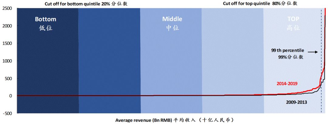
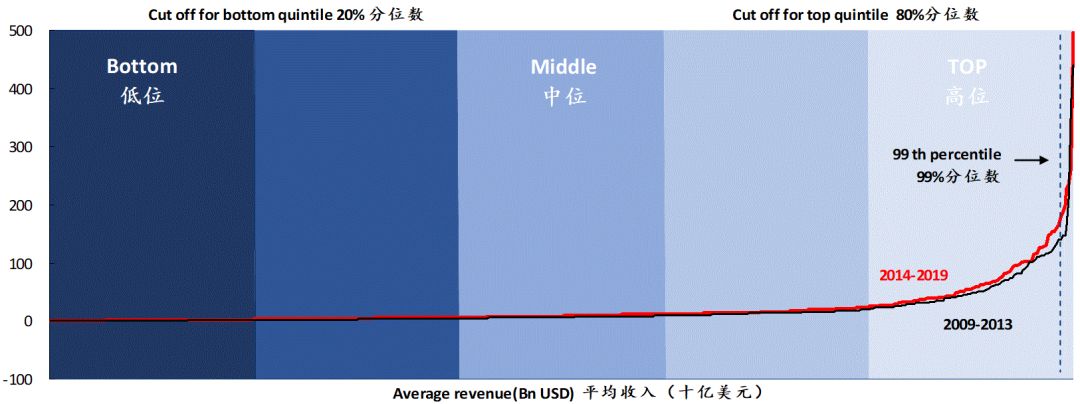
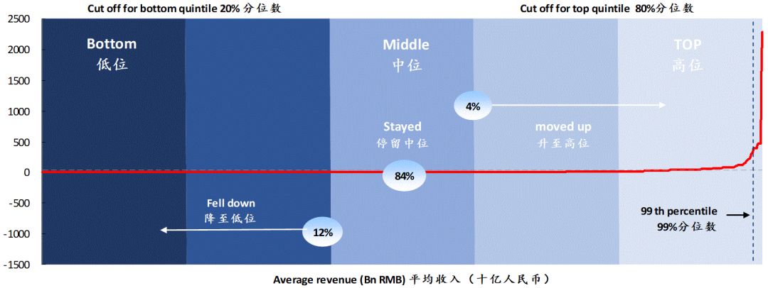
The reign of large caps will probably end once their return on equity falls below the discount rate. Further, our research shows that, in the past decade, leaders’ market power, as measured by their share in total industry revenue, has become even more concentrated (Figure 15). And once the industry structure is set, there is little mobility between different tiers of industry ranks. For instance, there is only a 4% chance for lower-ranked companies to move into the top rank in both the US and China (Figure 16).
As such, the relative performance of the large caps will likely persist for now, given their ROE above discount rate, increasing industry concentration, and limited mobility between ranks.
Figure 15: Industry concentration in both China and the US (bottom) increasing
Source: Bloomberg, BOCOM Int'l estimates
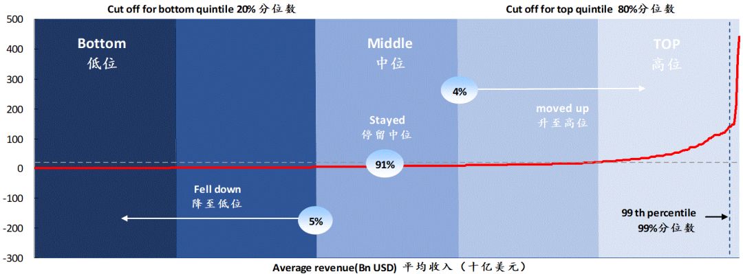
The reign of large caps will probably end once their return on equity falls below the discount rate. Further, our research shows that, in the past decade, leaders’ market power, as measured by their share in total industry revenue, has become even more concentrated (Figure 15). And once the industry structure is set, there is little mobility between different tiers of industry ranks. For instance, there is only a 4% chance for lower-ranked companies to move into the top rank in both the US and China (Figure 16).
As such, the relative performance of the large caps will likely persist for now, given their ROE above discount rate, increasing industry concentration, and limited mobility between ranks.
Figure 15: Industry concentration in both China and the US (bottom) increasing
 Source: Bloomberg, FactSet, Wind, BOCOM Int'l estimates
Figure 16: Mobility among industry ranks is limited in both China and US (bottom)
Source: Bloomberg, FactSet, Wind, BOCOM Int'l estimates
Figure 16: Mobility among industry ranks is limited in both China and US (bottom)
 Source: Bloomberg, FactSet, Wind, BOCOM Int'l estimates
Market Outlook
Our earning-yield-bond-yield model (EYBY) has a long and consistent forecasting track record. The trading range forecast for the Shanghai Composite in 2019, published in our outlook report titled “Outlook 2019: Turning a Corner” on 19 November 2018, was between 2,000 and 2,900, with 2,450 most likely to be bottom and 2,000 to be the extreme risk scenario with an event probability of 1%.
While the composite traded above 3,200 at its highest in April, in the past 12 months, the volume-weighted average of the composite’s trading range has been ~2,900, and ~80% of the time below 3,000, with the range between 2,900 and 3,000 being a significant resistance level. Further, the Shanghai Composite has really “turned a corner” in 2019, and is ranked one of the best-performing major indices in the world.
Indeed, we estimated the bottom for the composite at 2,450 in our report titled “Market Bottom: When and Where?” on 6 June 2016 – more than two years before the market eventually bottomed at 2,440 on 4 January 2019.
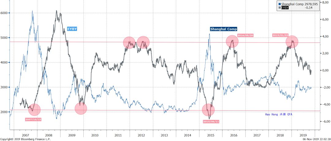
Given the track record of our EYBY model, we continue to apply it to forecasting 2020. We note that our EYBY model is now stuck at a neutral range that tended to linger for some time in history (Figure 17). This is a range where the Shanghai Composite tends to take a breather after a year of substantial move, and tries to reflect new data and information before resuming its uptrend, as the EYBY model grinds lower.
Figure 17: EYBY has reached a neutral trading range that used to persist for some time
Source: Bloomberg, FactSet, Wind, BOCOM Int'l estimates
Market Outlook
Our earning-yield-bond-yield model (EYBY) has a long and consistent forecasting track record. The trading range forecast for the Shanghai Composite in 2019, published in our outlook report titled “Outlook 2019: Turning a Corner” on 19 November 2018, was between 2,000 and 2,900, with 2,450 most likely to be bottom and 2,000 to be the extreme risk scenario with an event probability of 1%.
While the composite traded above 3,200 at its highest in April, in the past 12 months, the volume-weighted average of the composite’s trading range has been ~2,900, and ~80% of the time below 3,000, with the range between 2,900 and 3,000 being a significant resistance level. Further, the Shanghai Composite has really “turned a corner” in 2019, and is ranked one of the best-performing major indices in the world.
Indeed, we estimated the bottom for the composite at 2,450 in our report titled “Market Bottom: When and Where?” on 6 June 2016 – more than two years before the market eventually bottomed at 2,440 on 4 January 2019.
Given the track record of our EYBY model, we continue to apply it to forecasting 2020. We note that our EYBY model is now stuck at a neutral range that tended to linger for some time in history (Figure 17). This is a range where the Shanghai Composite tends to take a breather after a year of substantial move, and tries to reflect new data and information before resuming its uptrend, as the EYBY model grinds lower.
Figure 17: EYBY has reached a neutral trading range that used to persist for some time
 Source: Bloomberg, BOCOM Int'l estimates
For now, the Shanghai Composite is running into resistance defined by the 850-day moving average of ~3,200. This is a level that the moving average has been failing to break through since 2010 (Figure 13). That is, since 2010, the composite has been stuck in a range, as China’s saving-investment habit changes. China has been saving less, investing less and growing slower, as suggested by the country’s falling current account surplus to GDP ratio, money supply, FAI and IP. We have discussed these secular macro changes in our previous report titled “A Definitive Guide to Forecasting China Market” on 20 September 2019.
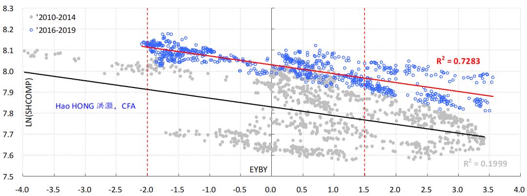
We have plotted EYBY and its corresponding composite levels on logarithmic scale in Figure 18. To eliminate the distortion from extreme data as the result of an abnormal trading year, we have excluded the data from 2015 – the year of stock market bubble. Further, we have grouped the data into pre- and post-bubble years starting from 2010 – the watershed year in the trading patterns in the Shanghai Composite discussed above.
As the Shanghai Composite has an internal compound rate of return that equals the economic growth target implicitly embedded in China’s Five-year Plan, the composite has a rising bottom that doubled every decade since 1996 (“The Market Bottom: When and Where?” 20160606). As such, we have explicitly based our 2020 forecast on the data points between 2016 and 2019 (Figure 18, blue dots). We believe EYBY will be stuck between the value of -2 and 1.5, given the inflation outlook and its implications for bond yield.
Consequently, the bottom trading range in 2020 is likely to be around 2,700, and 3,200 will remain a significant resistance for the 850-day moving average. It is likely that the moving average will continue to decline, if no exogenous factors are introduced into the Chinese market. The bottom level is calculated by growing the previous bottom of 2,450 by the EPS growth rate. Even if spot price temporarily surges above the 850-day moving average of 3,200, it is unlikely to change the top of the moving average established since 2010 – unless exogenous factor, such as significant foreign capital inflow, is introduced into the Chinese market. Not even the bubble in 2015 could change that.
Figure 18: The trading range = ~2,500-3,500; most likely bottom level = ~2,700
Source: Bloomberg, BOCOM Int'l estimates
For now, the Shanghai Composite is running into resistance defined by the 850-day moving average of ~3,200. This is a level that the moving average has been failing to break through since 2010 (Figure 13). That is, since 2010, the composite has been stuck in a range, as China’s saving-investment habit changes. China has been saving less, investing less and growing slower, as suggested by the country’s falling current account surplus to GDP ratio, money supply, FAI and IP. We have discussed these secular macro changes in our previous report titled “A Definitive Guide to Forecasting China Market” on 20 September 2019.
We have plotted EYBY and its corresponding composite levels on logarithmic scale in Figure 18. To eliminate the distortion from extreme data as the result of an abnormal trading year, we have excluded the data from 2015 – the year of stock market bubble. Further, we have grouped the data into pre- and post-bubble years starting from 2010 – the watershed year in the trading patterns in the Shanghai Composite discussed above.
As the Shanghai Composite has an internal compound rate of return that equals the economic growth target implicitly embedded in China’s Five-year Plan, the composite has a rising bottom that doubled every decade since 1996 (“The Market Bottom: When and Where?” 20160606). As such, we have explicitly based our 2020 forecast on the data points between 2016 and 2019 (Figure 18, blue dots). We believe EYBY will be stuck between the value of -2 and 1.5, given the inflation outlook and its implications for bond yield.
Consequently, the bottom trading range in 2020 is likely to be around 2,700, and 3,200 will remain a significant resistance for the 850-day moving average. It is likely that the moving average will continue to decline, if no exogenous factors are introduced into the Chinese market. The bottom level is calculated by growing the previous bottom of 2,450 by the EPS growth rate. Even if spot price temporarily surges above the 850-day moving average of 3,200, it is unlikely to change the top of the moving average established since 2010 – unless exogenous factor, such as significant foreign capital inflow, is introduced into the Chinese market. Not even the bubble in 2015 could change that.
Figure 18: The trading range = ~2,500-3,500; most likely bottom level = ~2,700
 Source: Bloomberg, BOCOM Int'l estimates
Within the broader market, our quantitative analysis shows that cyclicals have substantially underperformed defensive, and small caps underperformed large caps. Some traders may be tempted to take advantage of a technical rebound. But as our analysis above shows, the leading steers of their respective industries will continue to consolidate their market power, and thus increase industry concentration. Meanwhile, as global investment return continues to fall, as suggested by the falling EBITDA-to-capex ratio in the US, the secular underperformance of EM, cyclical and small caps is not yet over. In the long run, secular trends trump technical moves.
Source: Bloomberg, BOCOM Int'l estimates
Within the broader market, our quantitative analysis shows that cyclicals have substantially underperformed defensive, and small caps underperformed large caps. Some traders may be tempted to take advantage of a technical rebound. But as our analysis above shows, the leading steers of their respective industries will continue to consolidate their market power, and thus increase industry concentration. Meanwhile, as global investment return continues to fall, as suggested by the falling EBITDA-to-capex ratio in the US, the secular underperformance of EM, cyclical and small caps is not yet over. In the long run, secular trends trump technical moves.